Coherent Event Display
This page provides an overview of the coherent event display (CED). The CED is a web page providing a detailed description of a specific trigger reconstructed by cWB. The CED consists of a number of sections, with each section highlighting one different aspect of the reconstructed trigger. A detailed description of the different sections is available at the following links (the description is based on the CED of a SG849Q8d9 simulated signal
Note
All parameters and plots reported below are based on the CED of a SG849Q8d9 simulated signal
Job Parameters
This page provides a concise description of one of the sections in the coherent event display (CED). The section consists of a table summarising the job segment, the network, which search reconstructed the considered trigger and, if applicable, the MDC simulated signal. An example of this table is available below
NETWORK |
L1H1V1 |
SEARCH |
2G:MRA:Packet(+10) un-modeled(r) |
START SEGMENT |
931158370.000 |
STOP SEGMENT |
931158430.000 |
MDC |
SG849Q8d9 |
Event Parameters
This page provides a concise description of one of the sections in the coherent event display (CED). The section consists of a table listing the following trigger’s parameters as they were estimated by cWB:
SNR: network signal-to-noise ratio
rho: effective correlated amplitude (cWB test statistic)
cc: correlation coefficient (cWB test statistic)
ED: network energy disbalance (cWB test statistic)
PHI, THETA: source’s estimated sky coordinates (Earth frame)
An example of this table is shown below
GPS TIME |
SNR |
RHOi[0/1] |
CC[0/1/2/3] |
ED |
PHI |
THETA |
|---|---|---|---|---|---|---|
931158395.096 |
31.5 |
13.8/12.6 |
0.88/0.87/0.91/0.90 |
0.09 |
61.9 |
25.0 |
The whole list of the trigger’s parameters reconstructed by cWB is
available at the following link, reported on the CED page:
Estimated Parameters. An example of the list is reported below.
An explanation of each parameter is available here: trigger parameters
CED Estimated Parameters: Show/Hide Code
# WAT Version : 6.2.6.0 - GIT Revision : 4fbcbfa076e28b708291a754cbbe7981f2ef2210 - Tag/Branch : master/
# trigger 1 in lag 0 for
nevent:     1
ndim:       3
run:        1
name:       SG849Q8d9
rho:        13.800696
netCC:      0.878166
netED:      0.004591
penalty:    1.017278
gnet:       0.471306
anet:       0.459034
inet:       0.000000
likelihood: 9.934819e+02
ecor:       7.681392e+02
ECOR:       3.875000e+02
factor:     30.000000
range:      0.000000
mchirp:     0.000000
norm:       9.660262
usize:      0
ifo:        L1 H1 V1
eventID:    1 0
rho:        13.800696 12.552147
type:       1 3
rate:       0 0 0
volume:     415 200 0
size:       211 204 0
lag:        0.000000 0.000000 0.000000
slag:       0.000000 0.000000 0.000000
phi:        61.875000 60.000031 95.822701 61.875000
theta:      65.046982 60.000000 24.953020 65.046982
psi:        94.157990 89.999985
iota:       1.140301 0.000000
bp:         -0.4121  0.2246 -0.0082
inj_bp:     -0.3217  0.1569 -0.1341
bx:         -0.2455  0.2747  0.7376
inj_bx:     -0.2328  0.2214  0.7615
chirp:      0.000000 2.800020 0.024130 0.940894 0.875000 0.934442
range:      0.000000 0.000000
Deff:       0.000000 0.000000 0.000000
mass:       0.000000 0.000000
spin:       0.000000 0.000000 0.000000 0.000000 0.000000 0.000000
eBBH:       0.000000 0.000000 0.000000 0.000000
null:       1.130002e+01 3.298518e+01 1.486278e+01
strain:     1.731510e-22 4.159095e-22
hrss:       1.299835e-22 8.290716e-23 7.881598e-23
inj_hrss:   1.338139e-22 6.524630e-23 5.578825e-23
noise:      5.035646e-24 5.045541e-24 9.712598e-24
segment:    931158360.0000 931158440.0000 931158360.0000 931158440.0000 931158360.0000 931158440.0000
start:      931158394.7500 931158394.7500 931158394.7500
time:       931158395.1215 931158395.1181 931158395.0964
stop:       931158395.5000 931158395.5000 931158395.5000
inj_time:   931158395.1207 931158395.1173 931158395.0963
left:       34.750000 34.750000 34.750000
right:      44.500000 44.500000 44.500000
duration:   0.012848 0.750000
frequency:  834.093140 830.844849
low:        576.000000
high:       1088.000000
bandwidth:  54.934826 512.000000
snr:        7.740820e+02 2.218187e+02 1.033427e+02
xSNR:       7.159107e+02 2.436018e+02 8.122875e+01
sSNR:       6.621109e+02 2.675241e+02 6.384688e+01
iSNR:       696.472168 163.594635 32.708847
oSNR:       662.110901 267.524109 63.846878
ioSNR:      652.057068 197.664261 31.210590
netcc:      0.878166 0.872941 0.909277 0.897671
neted:      3.526730 153.305969 1099.243408 4678.104492 5416.478516
erA:         7.243  0.793  1.296  1.774  2.149  2.467  2.824  3.140  3.578  4.173 4200.657
sky_res:    0.458065
map_lenght: 179
#skyID  theta   DEC     step   phi     R.A    step  probability    cumulative
 56664   65.0   25.0    0.35   61.9   95.8    0.70  2.994807e-02  2.994807e-02
 55127   64.1   25.9    0.35   61.5   95.5    0.70  2.753293e-02  5.748100e-02
 57176   65.4   24.6    0.35   62.2   96.2    0.70  2.555657e-02  8.303757e-02
 ...
 48981   60.0   30.0    0.35   60.1   94.1    0.70  4.665694e-05  0.000000e+00
Reconstructed Detector Responses
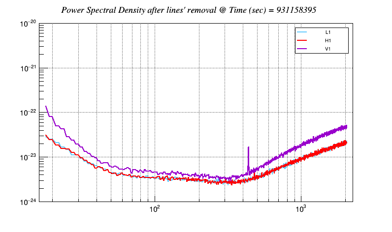
PSD
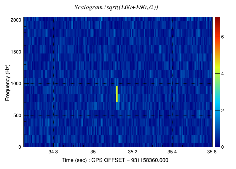
Time-Frequency Maps
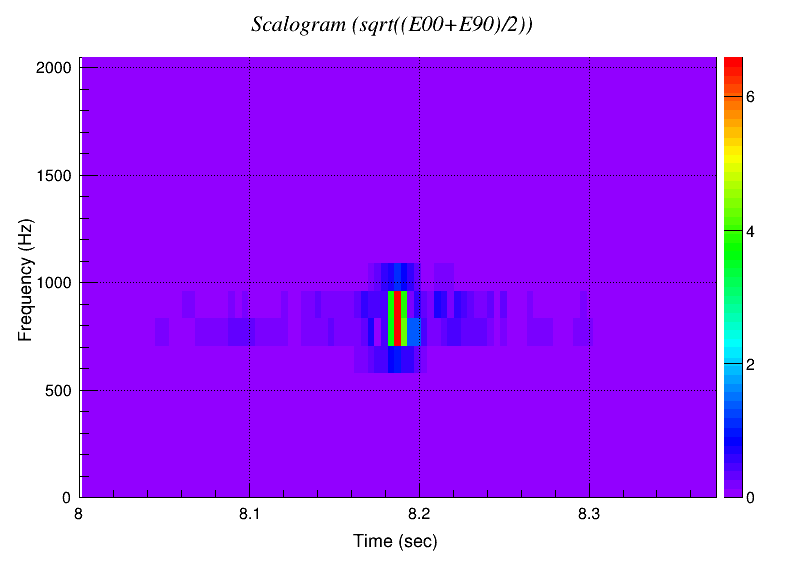
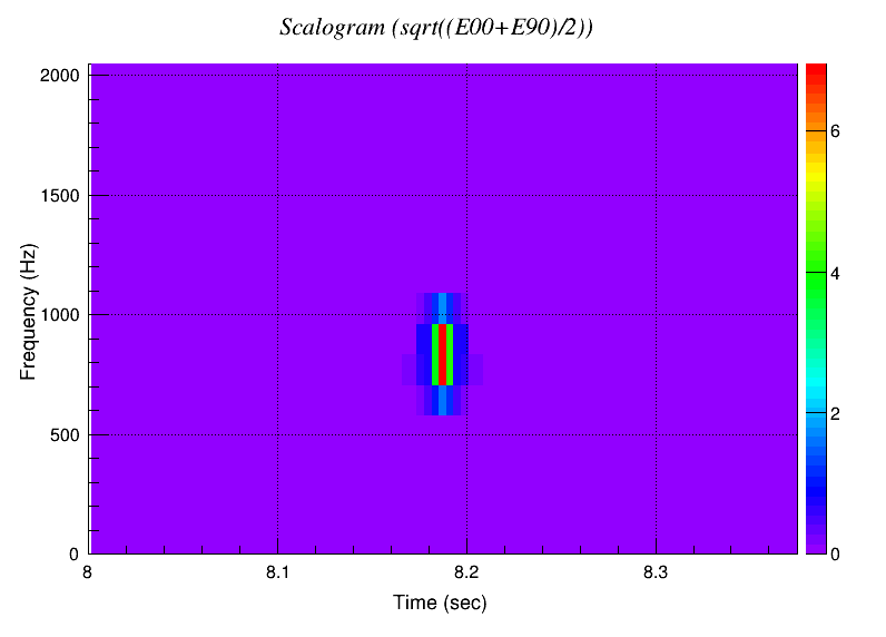
This page provides a concise description of one of the sections in the coherent event display (CED). The section shows the Time-Frequency (TF) maps of the reconstructed trigger. The TF maps describe how the trigger’s amplitude, normalised by the root mean square of the noise, is distributed over the considered area on the TF domain. The CED reports two different TF maps:
Spectrogram, showing a TF representation of the trigger, based on the Fourier decomposition.
Scalogram, showing the amplitudes of the wavelet coefficients (at the TF decomposition level at which the trigger has been reconstructed).
Both maps are generated for each detector in the network. Examples of the two different TF maps for the Livingston detector are reported below
Spectrogram

Scalogram
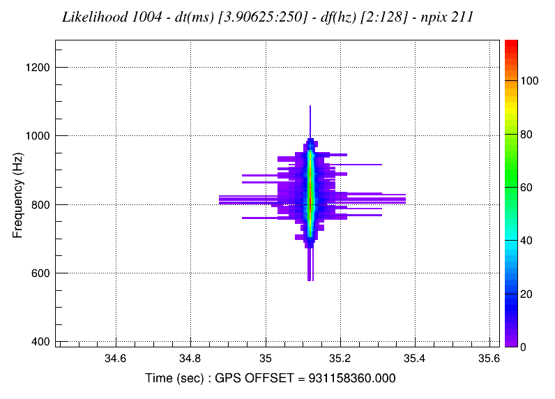
Likelihood Time-Frequency Maps
This page provides a concise description of one of the sections in the coherent event display (CED). The section shows the Time-Frequency (TF) maps of the two following network quantities:
Likelihood: contribution to the total energy content of the data stream associated to the reconstructed event (related to the network signal-to-noise ratio)
Null energy: contribution to the total energy content of the data stream associated to the null stream
Examples of the likelihood and null-energy TF maps are reported below
Likelihood Scalogram
Null Energy Scalogram

Reconstructed Detector Responses
This page provides a concise description of one of the sections in the coherent event display (CED). The section shows the reconstructed responses for each detector on the Time, Frequency and Time-Frequency domains. Three different plots are available:
Reconstructed signal (in the Time and Frequency domains)
Comparison between Signal and Noise (in the Time and Frequency domains)
Comparison between Reconstructed and Injected signal (only for the case of simulated signals)
Examples of the plots are reported below
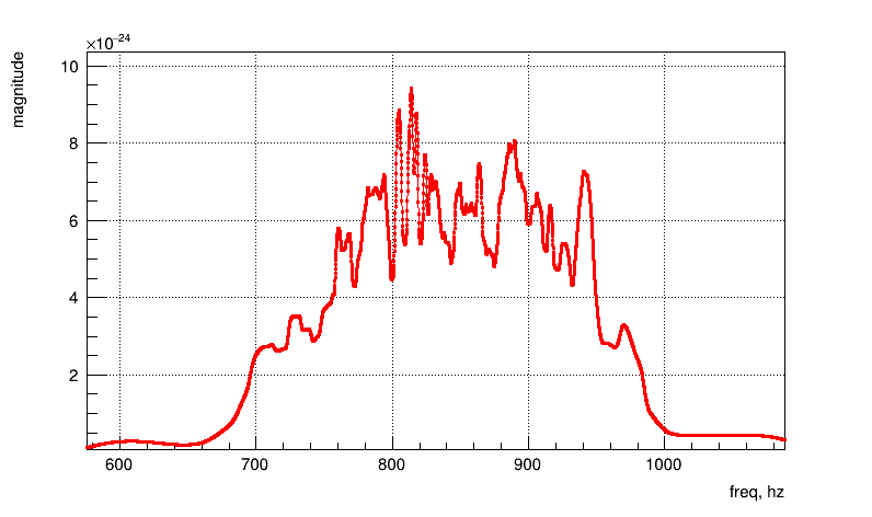
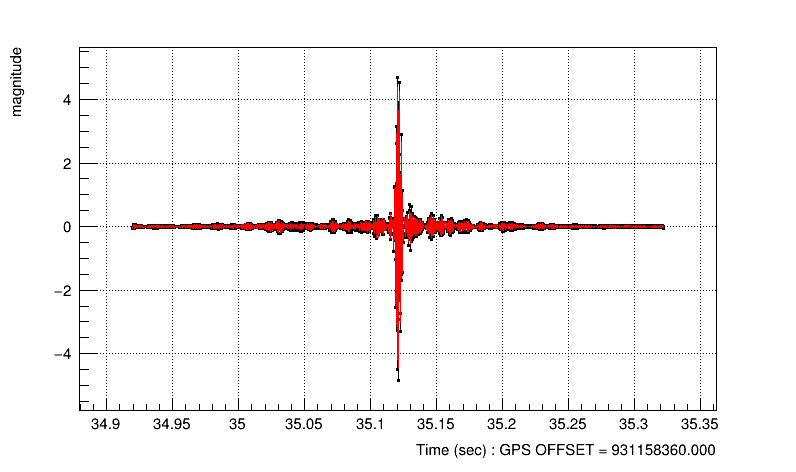
Reconstructed strain signal (in the Time and Frequency domains)
Time domain

Frequency domain
Signal/Noise comparison of whitened data
These plots show the reconstructed whitened signal (red) and the noise plus the reconstructed signal (black) in the Time and Frequency domains.
Time domain
Frequency domain

Comparison of the injected (red) and recovered (black) signals in the Time, Frequency and Time-Frequency domains (only for simulation studies)
Time domain
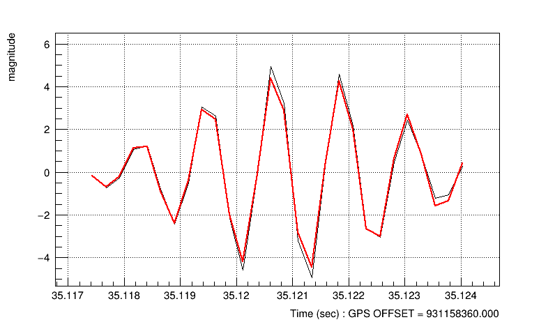
Frequency domain

Time-Frequency Reconstructed
Time-Frequency Injected
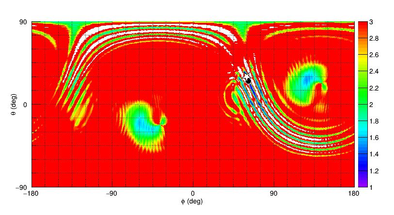
Skymaps
This page provides a concise description of one of the sections in the coherent event display (CED). The section reports Skymaps, which show how the values of the following quantities vary across the sky:
Sensitivity to the Plus Polarisation \(F_+^2\)
Sensitivity to the Cross Polarisation \(F_X^2\)
Sky statistics
Sky probability
Detection statistics
Likelihood
Null energy
Correlated Energy
Correlation
Likelihood Disbalance
Network response index
Polarization
Ellipticity
The Skymaps are calculated by using an Earth-fixed frame and enable the estimation of the source sky location, denoted by a black star. When performing simulation studies, the sky position of the injected signal is denoted by a white star to enable a straightforward comparison to the reconstructed source’s location.
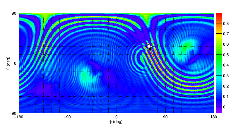
Sensitivity
This Skymap shows how the network sensitivity to the signal’s Plus and Cross polarizations varies across the sky. The sensitivity is estimated from the Plus and Cross network antenna patterns, calculated within the formalism of the Dominant Polarization Frame. The closer the antenna pattern is to one, the more sensitive the network is to the considered signal’s polarization. Examples of this Skymap are available below
Sensitivity to Plus Polarisation :math:`F_+^2`
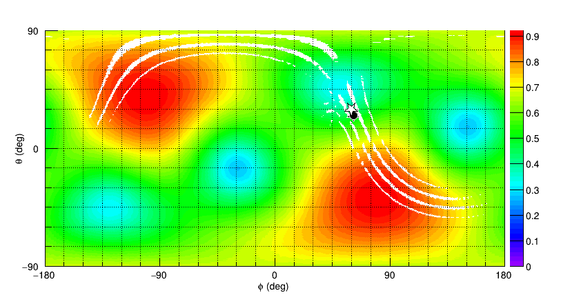
Sensitivity to Cross Polarisation :math:`F_X^2`

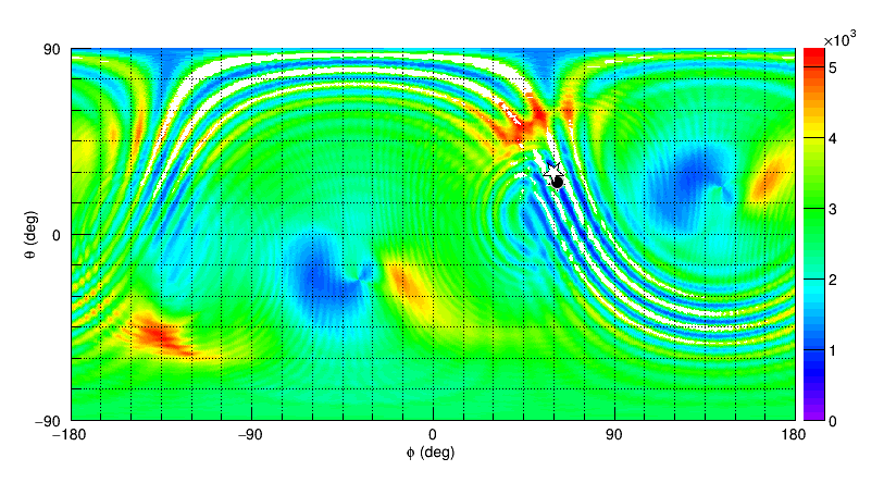
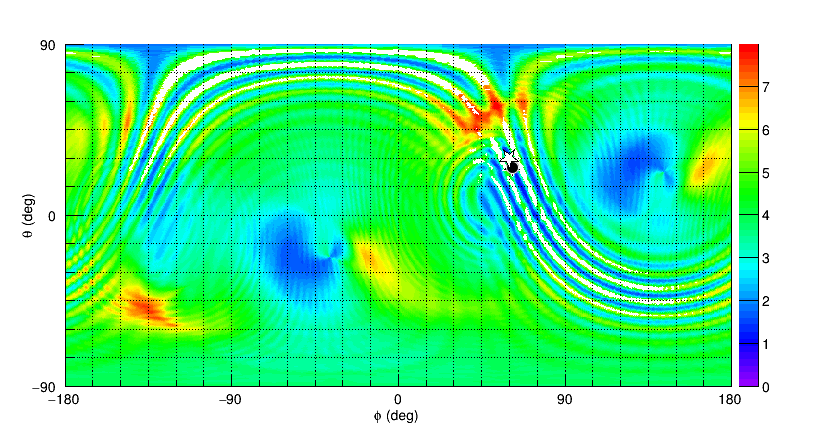
Sky and Detection statistics
These Skymaps show how the values of the Sky and Detection statistics vary across the sky. The Sky statistic is used to estimate the source’s location: the larger the Sky statistic over a given sky region, the higher the probability that the source is localised within the considered region. The Detection statistic is used to detect events and the consistency thresholds are based on the sky position at which the Detection statistic assumes the largest value. Examples of Sky and Detection Skymaps are available below
Sky Statistic

Sky probability
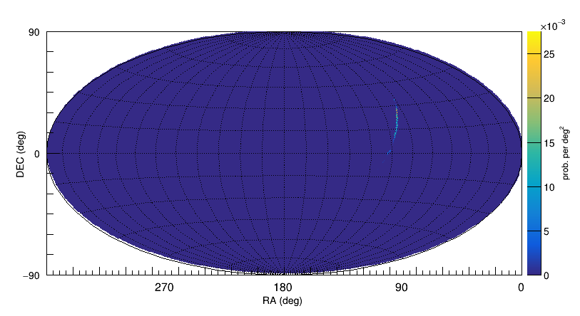
Detection Statistic
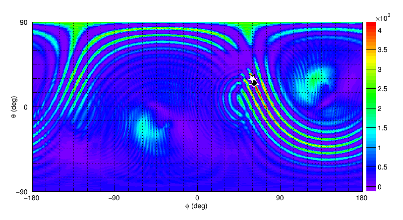
Event energy
These Skymaps show the variation across the sky of the Likelihood and Null Energy (see here: Likelihood Time-Frequency Maps for a definition of the two quantities). Examples of the Skymaps are shown below
Likelihood
Null Energy
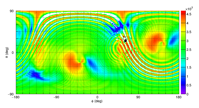
Correlation
This Skymap shows the variation across the sky of the Correlated Energy and of the Correlation coefficient. The Correlated Energy is an estimate of the signal’s energy content and is calculated from the correlation between the detectors. The Correlation Coefficient (cc) provides an estimate of the trigger’s coherence: whereas real gravitational-wave events should be identified with cc close to unity, events of noise origin should be characterised by cc values << 1. Thus, the larger is the value of cc, the more probable is that the considered trigger is a genuine gravitational wave. Examples of these Skymaps are available below
Correlated Energy

Correlation
Likelihood Disbalance and NRI
These Skymaps show how the values of the Likelihood disbalance and of the network response index vary across the sky. For a description of the Likelihood disbalance, see here. For a description of the network response index, see here.
Likelihood Disbalance
Network Detector Index