Graphical Library
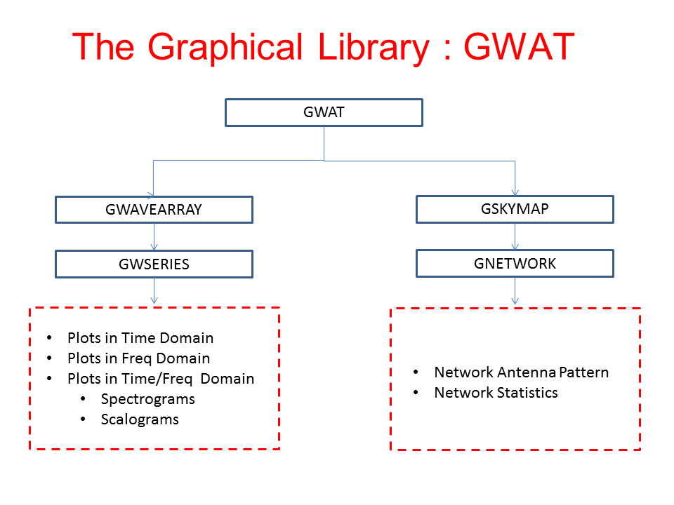
This page gives a concise description of the cWB graphical library (GWAT). The gwat classes provide a set of routines enabling the drawing of waveforms and skymaps. The different plots and classes which implement of the GWAT library are listed below:
gwavearray |
|
gWSeries |
|
gskymap |
|
detector’s network antenna pattern or the statistics produced in the likelihood stage |
gnetwork |
The above list is summarised by the following image:
Examples showing how to use the GWAT library are reported in the following directory in the git distribution:
tools/gwat/tutorialsgwavearray
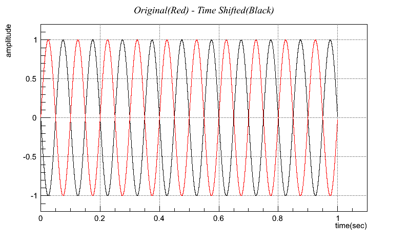
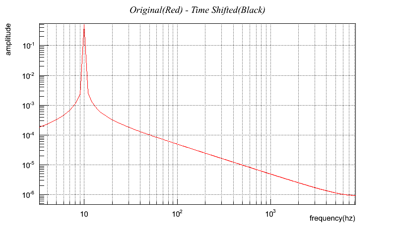
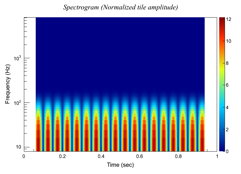
This page provides a description of the gwavearray class. This class is derived from the wavearray class and enables the production plots in the time, frequency and time-frequency domains of waveforms stored in a wavearray structure.
Example
An example of how to use the gwavearray class for the case of a sinusoidal waveform is available at the following link:
DrawGWaveArray.C
The most relevant lines in this example are the following:
gwavearray<double> gw(16384);     // instantiation with size 16384 samples
gw.rate(16384);                   // set sample rate = 16384 Hz
gw.start(0);                      // set start time = 0

// fill with a sinusoid  100 Hz
double dt=1/gw.rate();
for(int i=0;i<gw.size();i++) gw[i]=sin(2*PI*100*dt*i);

// draw methods

gw.Draw(GWAT_TIME);               // draw signal in time domain
gw.Draw(GWAT_FFT);                // draw signal in frequency domain
gw.Draw(GWAT_TF);                 // draw signal in time-frequency domain
The output plots are collected below.
gwseries
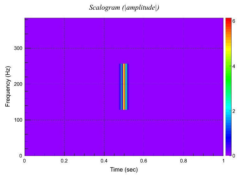
This page provides a description of the gWSeries class. This class is derived from the WSeries class and makes use of the scalogram plot and of the methods implemented in the gwavearray class.
Example
An example of how to use the gWSeries class is for the case of a sinusoidal waveform is available at the following link:
DrawGWSeries.C
The most relevant lines in this example are the following:
wavearray<double> x(16384);           // instantiation with size 16384 samples
x.rate(16384);                        // set sample rate = 16384 Hz
x.start(0);                           // set start time = 0

// add sin gaussian signal
double dt=1/x.rate();
double f=200;                         // frequency (Hz)
double s=0.01;                        // gaussian RMS
for(int i=0;i<x.size();i++) {
  int j=i-x.size()/2;
  x[i]=exp(-pow(dt*j,2)/2/s/s)*sin(2*PI*f*dt*j);
}

// do transformation level=8 and assign to gWSeries class
Meyer<double> S(1024,2);              // set wavelet for production
WSeries<double> w(x,S);
gWSeries<double> gw(w);               // assign to gWSeries class
gw.Forward(8);
cout << "level : " << gw.getLevel() << endl;

// plot scalogram
gw.DrawSG("FULL");                    // full time range
The output plot is shown below.
gskymap
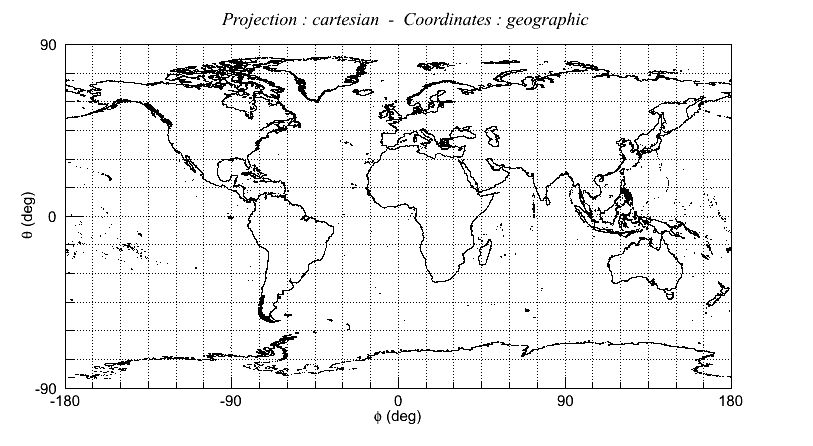
This page provides a description of the gskymap class. This class is derived from the skymap class and is used to generate the skymap plots.
Example
An example of how to use the gskymap class is available at the following link:
DrawGskymap.C
The most relevant lines in this example are the following:
// create gskymap with HEALPix order=7
gskymap gSM((int)7);

// set gskymap options
gSM.SetOptions("cartesian","geographic",1);

// set title
gSM->SetTitle("Projection : cartesian  -  Coordinates : geographic");

// set world map
gSM.SetWorldMap();

// draw skymap
gSM.Draw(0,"col");
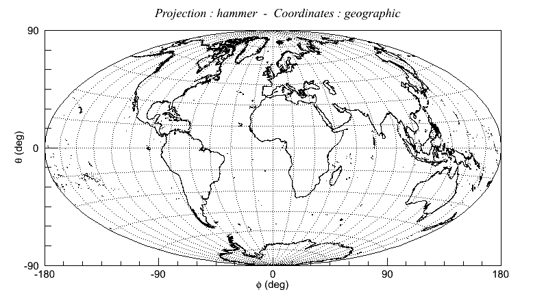
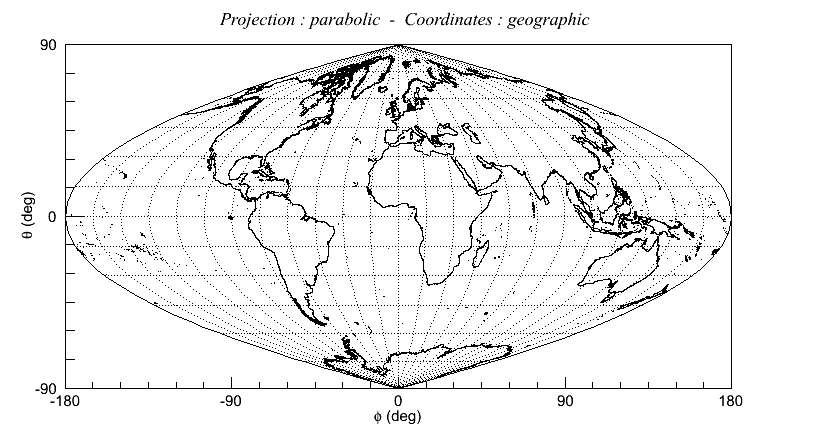
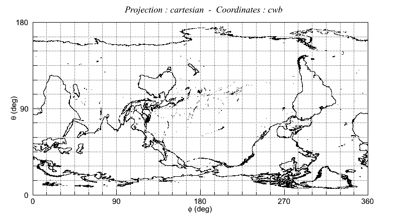
The different projections and coordinate frames available for this class generate the following plots:

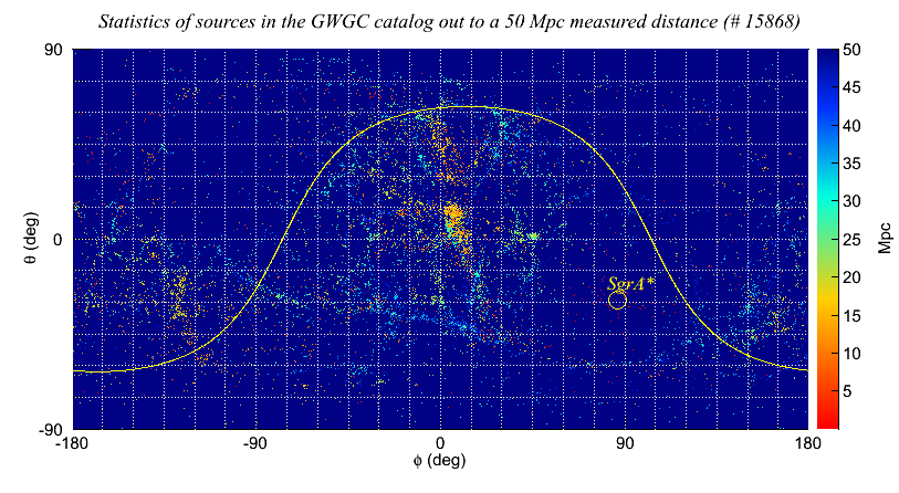
The following example shows how to produce “Statistics of sources in the GWGC catalog out to a %d Mpc measured distance 50Mpc”:
DrawGWGC.C
The output plot is reported below.
gnetwork
This page provides a description of the gnetwork class. This class is derived from the network class and uses the methods of the gskymap class. The gnetwork class is used to generate the skymaps of the detectors and networks’s antenna patterns or of the statistics calculated during the production stage of the cWB analysis
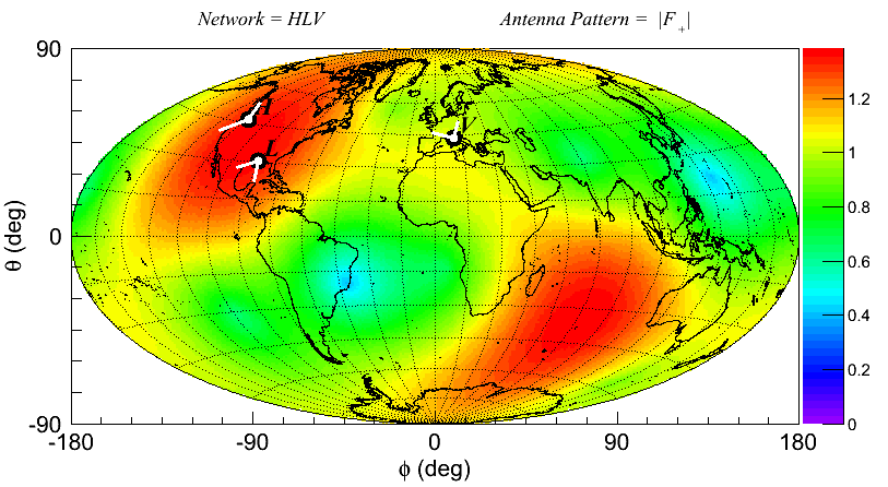
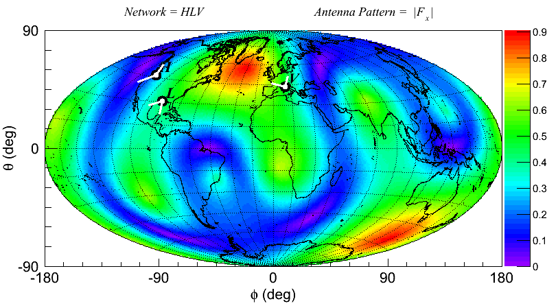
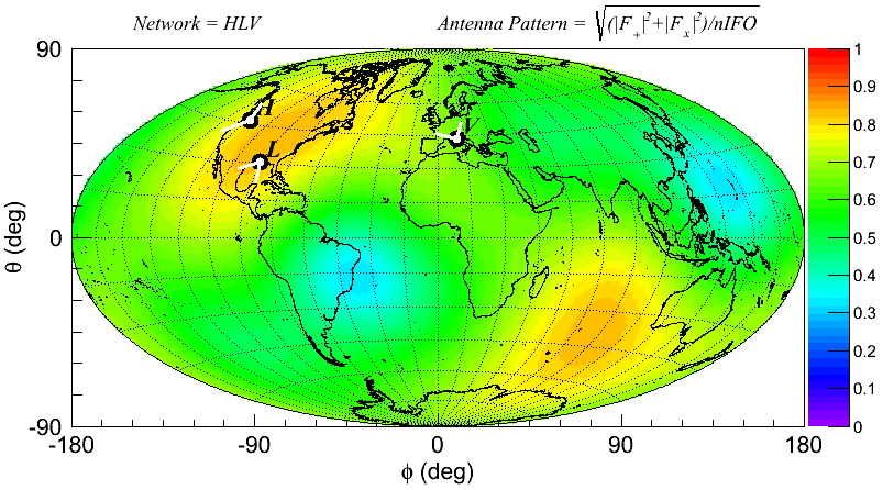
Method to draw the antenna pattern
The method to draw the detector and network antenna patterns is gnetwork::DrawAntennaPattern(int polarization=-1, int dpaletteId=0, bool btitle=true, int order=6) . Note that the antenna patterns are calculated in the Dominant Polarization Frame (DPF). The following quantities can be plotted by selecting the polarization parameter:
0 -> |Fx|                             - DPF
1 -> |F+|                             - DPF
2 -> |Fx|/|F+|                        - DPF
3 -> sqrt((|F+|^2+|Fx|^2)/nIFO)       - DPF
4 -> |Fx|^2                           - DPF
5 -> |F+|^2                           - DPF
6 -> Fx                               - only with 1 detector
7 -> F+                               - only with 1 detector
8 -> F1x/F2x                          - only with 2 detectors
9 -> F1+/F2+                          - only with 2 detectors
10 -> sqrt(|F1+|^2+|F1x|^2)/sqrt(|F2+|^2+|F2x|^2) - only with 2 detectors
11 -> The same as (10) but averaged over psi      - only with 2 detectors
Method to draw the network likelihood statistics
The method to draw the network likelihood statistics calculated during the production stage of the cWB analysis is gnetwork::Draw(TString smName, network *net=NULL) . The smName parameter can be as follows:
nSensitivity   : network sensitivity
nAlignment     : network alignment factor
nCorrelation   : network correlation coefficient
nLikelihood    : network likelihood
nNullEnergy    : network null energy
nPenalty       : signal * noise penalty factor
nCorrEnergy    : reduced correlated energy
nNetIndex      : network index
nDisbalance    : energy disbalance
nSkyStat       : sky optimization statistic
nEllipticity   : waveform ellipticity
nPolarisation  : polarisation angle
nProbability   : probability skymap

index          : theta, phi mask index array
skyMask        : index array for setting sky mask
skyMaskCC      : index array for setting sky mask Celestial Coordinates
skyHole        : static sky mask describing "holes"
veto           : veto array for pixel selection
skyProb        : sky probability
skyENRG        : energy skymap
Example
An example of how to use the gnetwork class is available at the following link:
DrawAntennaPattern.C
The most relevant lines in this example are the following:
// create gnetwork
gnetwork gNET;

// add detectors to gnetwork
int nIFO=3;
TString ifo[3]={"L1","H1","J1"};
detector* pD[3];
for(int i=0; i<nIFO; i++) pD[i] = new detector(ifo[i].Data()); // built in detector
for(int i=0; i<nIFO; i++) gNET.add(pD[i]);

gskymap* gSM = gNET.GetGskymap();
// set graphical options
gSM->SetOptions("cartesian","geographic",1);
// set world map
gSM->SetWorldMap();

// draw Antenna Pattern (show title)
gNET.DrawAntennaPattern(1,0,true);
// draw site labels
gNET.DrawSitesShortLabel(kBlack);
// draw site markers
gNET.DrawSites(kBlack,2.0);
// draw site arms
gNET.DrawSitesArms(1000000,kWhite,3.0);
The output plots are shown below.