XGBoost with cWB
References
What is eXtreme Gradient Boosting (XGBoost)
eXtreme Gradient Boosting |
|
Veto Method Limitations |
Enhancing cWB with XGBoost
Overall idea for integration of XGBoost into cWB |
|
List of input features (cWB summary statistics) for XGBoost |
|
XGBoost Ranking Statistic |
XGBoost Model Implementation ->
Setting up cWB working directories, data splitting for XGBoost training and testing |
|
Finding the most optimal XGBoost hyper-parameters set |
|
Creating and Storing the XGBoost model |
|
Predicting and estimating the significance using the stored XGBoost model |
|
Creating the final report page and additional plotting options |
XGBoost - eXtreme Gradient Boosting
Introduction
|
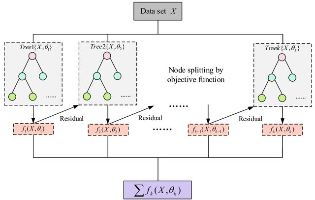
XGBoost flow chart for building an ensemble of trees. For a given dataset X, XGBoost builds subsequent trees by learning the residual of the previous tree as the input for the next tree [image credit].
Why XGBoost?
Veto method and its limitations
XGBoost Classifier
Enhancing cWB with XGBoost
Method
Reduced Detection Statistic
Post-O3 approach
O4 approach
For more information please check the papers linked here - 1, 2, 3, 4.
XGBoost model implementation
Data Splitting
Setting up the working directories
- We start by setting up 3 directories:
BKG - To store the Background data for each chunk involved in the XGBoost model.
SIM - To store the Simulations data.
XGB - To store the trained XGBoost model.
Clone working directories for XGBoost use by utilizing the cwb_clonedir command (for simulation directories add option ‘ –simulation true’ while cloning). This step is optional; XGBoost analysis can be performed in the original working directories as well.
cwb_clonedir /in_path_BKG/BKG_dir   /out_path/BKG/BKG_dir_xgb1   '--output smerge --label M1.V_hvetoLH'
cwb_clonedir /in_path_SIM/SIM_dir   /out_path/SIM/SIM_dir_xgb1   '--output smerge --label M1.C_U.V_hvetoLH --simulation true'
Create the XGB directory using cwb_mkdir /out_path/XGB/Model_dir_XGB.
XGB cuts
- Frequency cuts are applied prior to XGBoost processing. The frequency cuts are different for different search configurations:
BBH configuration: 60 Hz < \(f_0\) < 300 Hz
IMBH configuration: \(f_0\) < 200 Hz
BurstLF configuration: 16 Hz < \(f_0\) < 2048 Hz
The wave root files get a label xgb_cut at the end to denote that the frequency cut has been applied on those files.
cwb_setcuts M1.V_hvetoLH '--wcuts ((frequency[0]>60&&frequency[0]<300)&&(!veto_hveto_H1&&!veto_hveto_L1)) --label xgb_cut'
Data split
- We split the data for training and testing.
BKG data - For each chunk of available background data (usually around a 1000 years unless the chunk hosts some special GW events), 100 years of background data is kept for training, and the remaining data is set aside for testing.
SIM data - For every 100 years of background data that is used for training, we split 1000 simulation events for training and keep the rest of the simulation events for testing purposes.
The datasplit option is utilized for splitting the data with an option –ifrac which allows us to choose whether we want to split the root files based on number of years for BKG/events for SIM (
--ifrac -x, where x is an integer and x > 1) or based on the fraction of root events stored (--ifrac y, where 0 < y < 1).
cwb_xgboost datasplit '--mlabel M1.V_hvetoLH.C_xgb_cut --ifrac -100 --verbose true --cfile $CWB_CONFIG/O3a/CHUNKS/BBH//Chunk_List.lst'
The –cfile option points to the GPS times for the chunks available in order to assign the respective chunk numbers \(C_n\).
After the split we end up with two new wave root files for training and testing purposes.
- Create the following files in the XGB directory for tuning and training:
nfile.py - Input background files (wave_*.root/.py) for training.
sfile.py - Input simulation files (wave_*.root/.py) for training.
Note
cwb_xgboost_config.py script is used as the default input XGBoost configuration for tuning/training/prediction/report functionalities of the cwb_xgboost command. The default config values and options can be changed by including user defined user_xgboost_config_ .py files in the cwb_xgboost command options. The cwb_xgboost_config.py script is included at the end of this page for completion.
Tuning
XGBoost hyper-parameters |
entry |
learning_rate |
0.03, 0.1 |
max_depth |
13 |
min_child_weight |
10.0 |
colsample_bytree |
1.0 |
subsample |
0.4, 0.6, 0.8 |
gamma |
2.0, 5.0, 10.0 |
Sample Weight options
Apart from the XGBoost hyper-parameters, there are some user defined hyper-parameters that control the shape of a custom \(\eta_0\) dependent sample weight which is applied to the background events to minimize the importance given by the algorithm to low SNR glitches. All the simulation events are assigned a sample weight of 1. In contrast, for the noise events, we first divide simulation events in the interval \(6.5 < \eta_0 < 20\) into \(nbins\) = 100 percentile bins such that the number of simulation events in each bin is the same. The lower threshold at \(\eta_0\) = 6.5 gets rid of excess background with minimal or no loss of simulated events. The capping at \(\eta_0\) = 20.0 prevents the algorithm from being affected by high SNR background events.
Sample weight \(w\): For simulation events — \(w_{S} = 1\). For background events:
\[w_{B}(i) = \frac{N_{S}(i)}{N_{B}(i)}\, e^{\ln(A)\left(1-\frac{i}{nbins}\right)^q}\]where \(i = 1, 2, \ldots, nbins\) is a given bin, \(N_{S}(i)\) and \(N_{B}(i)\) are the number of simulation and background events in the \(i\)-th bin. \((q, A)\) are weight options where \(A\) is called the balance parameter — \(A = \frac{N_{S}(1)}{N_{B}(1)}\) is the class balance (\(N_{S}/N_{B}\)) for the first bin at \(\eta_0 \geq 6.5\) — and \(q\) is called the slope parameter that controls the rate of change of the weighted background distribution (defined in Mishra et al. 2022). For all events with \(\eta_0 \geq 20\), the number of simulation events is re-sampled to match the number of background events to have a perfect class balance (\(N_{S}/N_{B} = 1\)). For a given combination of \((q, A)\) values, we can achieve any monotonic distribution of our choice.
XGBoost hyper-parameters |
entry |
weight balance |
\(A\) = 40 |
weight slope |
\(q\) = 5 |
Show/Hide distribution of background events and simulation events after application of sample weight
|
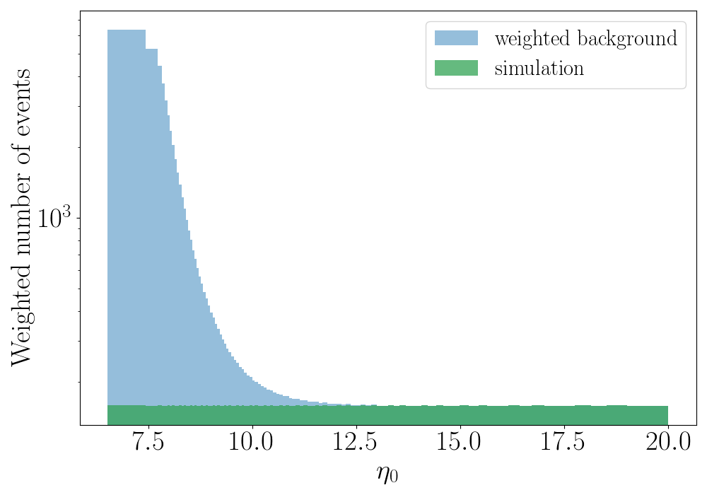
\(\eta_0\) dependent sample weight - Distribution of weighted background events and simulation events in the range \(6.5 < \eta_0 < 20\) after the application of sample_weight with (\(q\) = 5, \(A\) = 40).
The user_pparameters.C file is modified for tuning and the commands for tuning are as follows:
cwb_condor xgb r1
cwb_xgboost report '--type tuning --ulabel r1 --verbose true'
Show/Hide user_pparameters.C file
user_pparameters.C -

 // ----------------------------------------------------------
 // XGB parameters used for Tuning
 // ----------------------------------------------------------

 // This is an example which shows how to setup XGB in the user_pparameters.C file

 {

   // tuning/training/prediction
   pp_xgb_search         = "bbh";				// input search type (bbh/imbhb/blf/bhf/bld)

   // tuning
   pp_xgb_ofile          = "xgb/r1/tuning.out";			// output XGB hyper-parameters file

   // tuning/training
   pp_xgb_nfile          = TString(work_dir)+"/nfile.py";	// input background file (wave_*.root/.py)
   pp_xgb_sfile          = TString(work_dir)+"/sfile.py";	// input simulation file (wave_*.root/.py)
   pp_xgb_nfrac          = 0.2;					// input fraction of events selected from bkg
   pp_xgb_sfrac          = 0.2;					// input fraction of events selected from sim
 //  pp_xgb_config         = "$CWB_SCRIPTS/cwb_xgboost_config.py"; // input XGB configuration
 								// if not provided then the default config cwb_xgboost_config.py is used

   pp_xgb_config         = "config/user_xgboost_config_r1.py";   // input XGB configuration, leave empty if there are no changes needed

   // XGB hyper-parameters (tuning)

   // r1
   pp_xgb_learning_rate    = { 0.03 };
   pp_xgb_max_depth        = { 13 };
   pp_xgb_min_child_weight = { 10.0 };
   pp_xgb_colsample_bytree = { 1.0 };
   pp_xgb_subsample        = { 0.6 };
   pp_xgb_gamma            = { 2.0 };
   pp_xgb_balance_balance = { "A=1", "A=5", "A=20", "A=40", "A=100", "A=300", "A=500" };
   pp_xgb_balance_slope = { "q=0.5", "q=0.75", "q=1.0", "q=1.5", "q=2.0", "q=2.5", "q=3.0", "q=5.0", "q=10.0" };
   pp_xgb_caps_rho0 = { 20 };

   // used as input by the "cwb_condor xgb" command
   // can be also defined in user_parameters.C file
   strcpy(condor_tag,"ligo.prod.o3.burst.bbh.cwboffline");

 }
Training
/out_path/XGB/model_dir_XGB/config/user_xgboost_config_v1.py
Show/Hide user_xgboost_config_v1.py file
 ML_caps['rho0'] =  20                          #set the cap value for rho0 or eta_0, can be used to set cap value for other summary statistics
 ML_balance['slope(training)']     = 'q=5'      #set the weight slope hyper-parameter
 ML_balance['balance(training)']   = 'A=40'     #set the weight balance hyper-parameter

 ML_list.remove('Lveto2')                       #remove any cWB summary statistic from the input features list

 import cwb_xgboost as cwb
 ML_list.append(cwb.getcapname('norm',13))      #add any cWB summary statistic along with cap value for that statistic

 ML_options['rho0(mplot*d)']['enable'] = True   #1d and 2d hist plots
 ML_options['Qa(mplot*d)']['enable'] = True
 ML_options['Qp(mplot*d)']['enable'] = True     #similarly for other summary statistics

 ML_options['bkg(mplot2d)']['rho_thr'] = 15     #bkg minimum rho0 threshold for plotting on 2d hist

 ML_options['sim(mplot2d)']['cmap'] = 'rainbow' #color map for sim in the 2d hist
cwb_xgboost training '--nfile nfile.py --sfile sfile.py  --model xgb/v1/xgb_model_name_v1.dat --nfrac 1.0 --sfrac 1.0 --search bbh --verbose true --dump true --config config/user_xgboost_config_v1.py'
cwb_mkhtml xgb/v1/                     //(plots stored in public_html training report page in ldas)
A few example plots stored in the training report page
Show/Hide training report page plots
|

Last Tree Generated - Illustration of the last tree generated in the ensemble before training procedure stops.
|
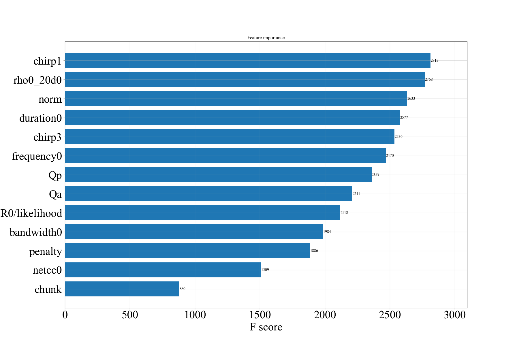
Feature importances - Importance of input features/summary statistics in training the XGBoost model.
|
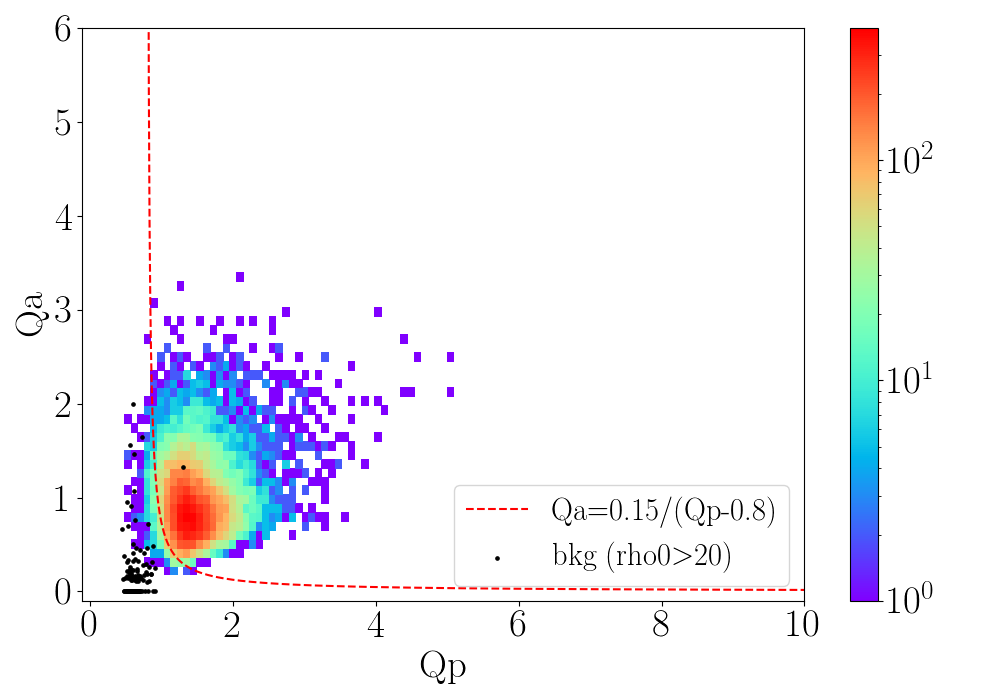
\(Q_a\) vs \(Q_p\) training plot - 2d hist plot of \(Q_a Q_p\) with scatterplot of high SNR background events.
|
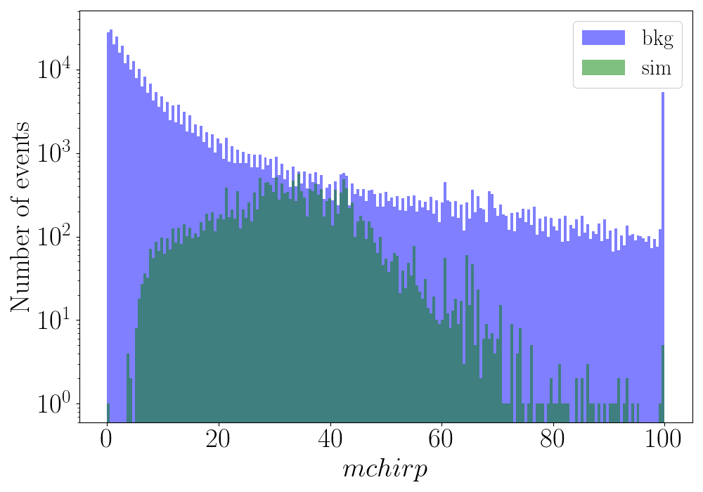
Chirp mass \(\mathcal{M}\) - Distribution of \(\mathcal{M}\) or mchirp for training background and simulation events.
|
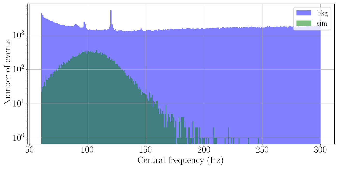
Central frequency \(f_0\) - Distribution of central frequency \(f_0\) for training background and simulation events.
|
\(\eta_0\) - Distribution of \(\eta_0\) or \(\rho_0\) for training background and simulation events.
If ML_options['enable_shap'] is set to True in the config file, the training
also produces a set of SHAP (SHapley Additive
exPlanations) diagnostic plots alongside the model: a clustered bar chart of
feature importance, a scatter plot of SHAP values per feature, and the
summary bar/beeswarm plots, saved next to the trained model with the
_shap_values*.png suffix.
The rho0(define) option, used to select the \(\rho_0\) definition,
now accepts two additional values besides the existing 0 (rho0 =
rho[0]) and 1 (rho0 = sqrt(ecor/(1+penalty*(max(1,penalty)-1)))):
2: \(\rho_0 = \sqrt{ecor}\)3: \(\rho_0 = \sqrt{likelihood}\)
Testing
BACKGROUND
/out_path/BKG/BKG_dir_xgb1 - For each chunk of background data, we go to the respective working directory and run the following commands:
Standard Veto Method for comparison
cwb_setcuts M1.V_hvetoLH.C_xgb_cut.XK_Test_Y100_TXXXX '--tcuts bin1_cut --label bin1_cut'
cwb_report M1.V_hvetoLH.C_xgb_cut.XK_Test_Y100_TXXXX.C_bin1_cut create
Prediction with XGBoost
cwb_xgboost M1.V_hvetoLH.C_xgb_cut.XK_Test_Y100_TXXXX '--model /out_path/XGB/model_dir_XGB/xgb/v1/xgb_model_name_v1.dat --ulabel v1 --rthr 0 --search bbh'
cwb_report M1.V_hvetoLH.C_xgb_cut.XK_Test_Y100_TXXXX.XGB_rthr0_v1 create
SIMULATION
/out_path/SIM/SIM_dir_xgb1 - For each simulation directory, we run the following commands:
Standard Veto Method for comparison
#set standard PP cuts
cwb_setcuts M1.C_U.V_hvetoLH.C_xgb_cut.XK_Test_NXX_TXXX '--tcuts bin1_cut --label bin1_cut'

#set ifar chunkwise, far_bin1_cut_file pointing to the standard far_rho.txt files for the respective BKG chunk
cwb_setifar M1.C_U.V_hvetoLH.C_xgb_cut.XK_Test_NXX_TXXX.C_bin1_cut        '--tsel O2_K01_cut --label ifar --file far_bin1_cut_file[1]  --mode exclusive'
cwb_setifar M1.C_U.V_hvetoLH.C_xgb_cut.XK_Test_NXX_TXXX.C_bin1_cut.S_ifar '--tsel O2_K02_cut --label ifar --file far_bin1_cut_file[2]  --mode exclusive'
#... so on for all the chunks.
Prediction with XGBoost
/out_path/SIM/SIM_dir_xgb1/config/user_pparameters.C
Show/Hide user_pparameters.C for setting IFAR
  // XGB
  #define nCHUNKS       X
  // read far vs rho background files
  TString xgb_far_bin1_cut_file[1024];
  vector<TString> xgb_xfile = CWB::Toolbox::readFileList("/out_path/BKG/XGB/far_rho_v1.lst");
  for(int n=0;n<xgb_xfile.size();n++) xgb_far_bin1_cut_file[n+1]=xgb_xfile[n];
  if(xgb_xfile.size()!=nCHUNKS) {
     cout << endl;
     for(int n=0;n<xgb_xfile.size();n++) cout << n+1 << " " << xgb_far_bin1_cut_file[n+1] << endl;
     cout << endl << "user_pparameters.C error: config/far_rho.lst files' list size must be = "
          << nCHUNKS << endl << endl;
     exit(1);
  }
#prediction
cwb_xgboost M1.C_U.V_hvetoLH.C_xgb_cut.XK_Test_NXX_TXXX '--model /out_path/XGB/model_dir_XGB/xgb/v1/xgb_model_name_v1.dat --ulabel v1 --rthr 0 --search bbh'

#set ifar
cwb_setifar M1.C_U.V_hvetoLH.C_xgb_cut.XK_Test_NXX_TXXX.XGB_rthr0_v1        '--tsel O2_K01_cut --label ifar --file xgb_far_bin1_cut_file[1]  --mode exclusive'
cwb_setifar M1.C_U.V_hvetoLH.C_xgb_cut.XK_Test_NXX_TXXX.XGB_rthr0_v1.S_ifar '--tsel O2_K02_cut --label ifar --file xgb_far_bin1_cut_file[2]  --mode exclusive'
#... so on for all the chunks.
sfile_rhor_v1.py - list of all the predicted root files using XGBoost for all simulation directories used (reduced detection statistic, rhor or \(\eta_r\)).
sfile_rho1.py - list of all the standard PP cuts root files for all simulation directories used (standard detection statistic, rho1 or \(\eta_1\)).
Report
/out_path/SIM/SIM_dir_test/report_config_v1.py
Show/Hide report_config_v1.py for setting IFAR
#Plot the roc - detection efficiency vs far (yr)
PLOT['roc']  = ['xgb/v1/roc.png','','']
ROC['rhor'] = ['sfile_rhor_v1.py','red']
ROC['rho1'] = ['sfile_rho1.py','blue']

#Plot detetion efficiency @IFAR 1yr vs the central frequency freq[0]
PLOT['efreq']  = ['xgb/v1/efreq.png','','',20,204,44,1]
EFREQ['rho_r'] = ['sfile_rhor_v1.py','red']
EFREQ['rho_1'] = ['sfile_rho1.py','blue']

#Plot the 1d histogram of rhor for both sim and bkg
PLOT['hrho'] = ['xgb/v1/hrhor.png','','r$\rho_r$']
HRHO['sim'] = ['sfile_rhor_v1.py',1,'green']
HRHO['bkg'] = ['/out_path/BKG/XGB/nfile_bkg_rhor_v1.py',1,'blue']

#Plot of log10(rhor) vs 0.5*log10(likelihood) with bkg points plotted for rhor> 8
PLOT['lrho'] = ['xgb/v1/lrhor.png','','r$\rho_r$']
LRHO['sim'] = ['sfile_rhor_v1.py',1,'green']
LRHO['bkg'] = ['/out_path/BKG/XGB/nfile_bkg_rhor_v1.py',1,'blue',8]


PLOT['qaqp'] = ['xgb/v1/qaqp_rthr8.png','rho1',8,'rhor',0.15,0.8]
QAQP['sim'] = ['sfile_rhor_v1.py']
QAQP['bkg'] = ['/out_path/BKG/XGB/nfile_bkg_rhor_v1.py']
cwb_xgboost report  '--type prediction --subtype roc/hrho/efreq/lrho/qaqp --config report_config_v1.py '
cwb_mkhtml xgb/v1/
Plots in the final XGBoost report page
|
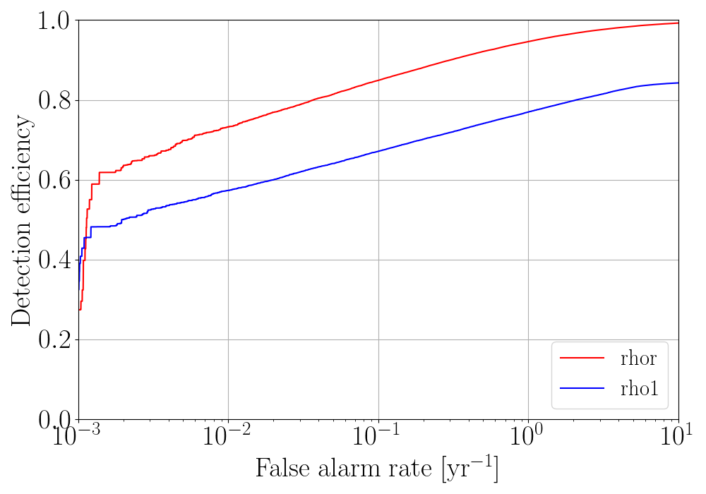
roc - Detection efficiency vs FAR plot for the ML-enhanced cWB search compared with the standard cWB search.
Show/Hide other important plots from the testing report page
|
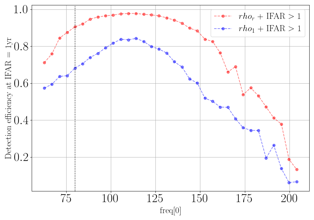
efreq - Detection efficiency @IFAR 1 yr vs central frequency \(f_0\) (or freq[0]) for the ML-enhanced cWB search compared with the standard cWB search.
|
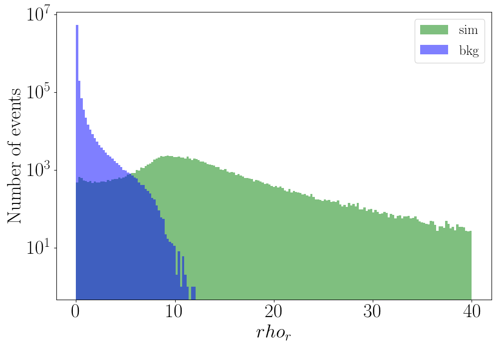
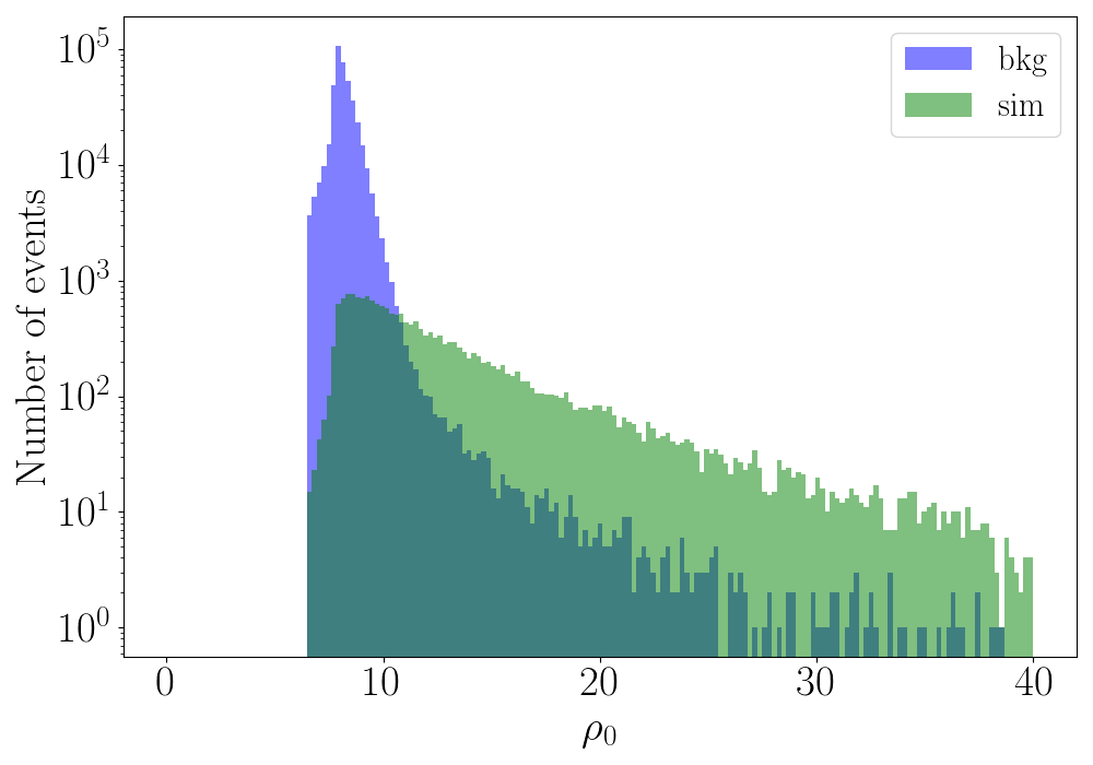
hrhor - Distribution of \(\eta_r\) or \(\rho_r\) for testing background and simulation events.
|
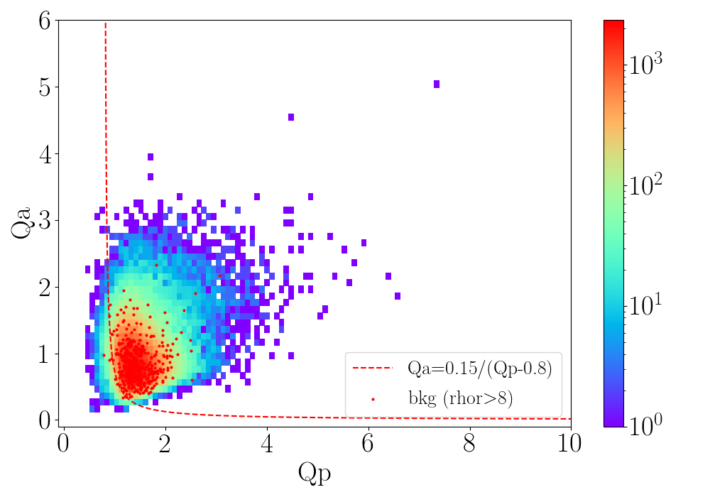
qaqp - 2d hist plot of \(Q_a\) vs \(Q_p\) with scatterplot of high SNR background events for testing events.
|
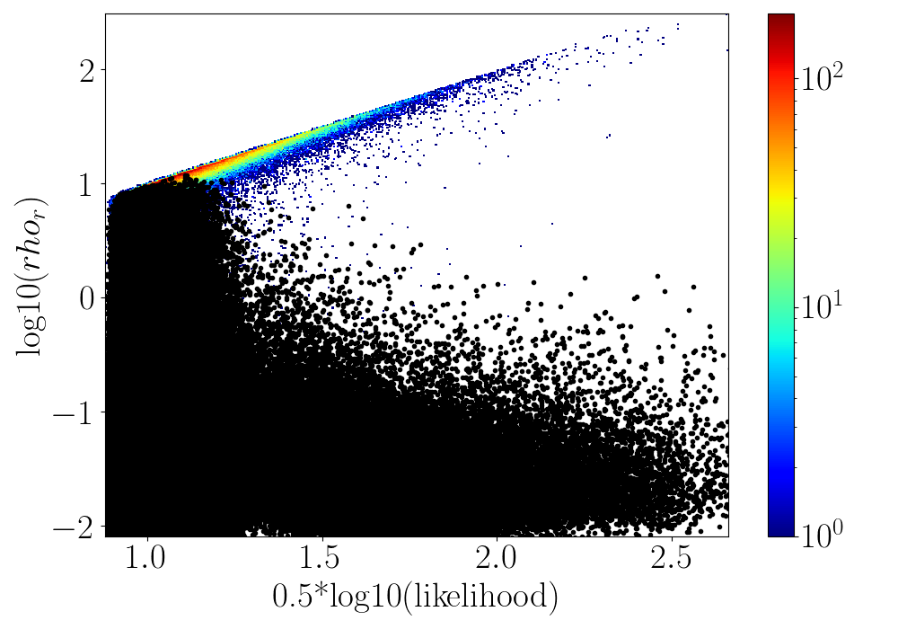
lrhor - \(\log_{10}(\eta_r)\) or \(\log_{10}(\rho_r)\) vs \(0.5 \cdot \log_{10}(\text{likelihood})\) for testing simulation events and scatterplot of high SNR testing background events.
cWB Summary Statistics
- The following 14 cWB summary statistics were used as the input features for the XGBoost BBH search and IMBH search models:
\(\eta_0\): The effective correlated SNR and the main cWB detection statistic used for the generic GW search. As an input feature for XGBoost, the \(\eta_0\) statistic is capped at 20 (any event with higher \(\eta_0\) is assigned the value 20). The capping prevents the algorithm from being affected by high SNR background events, which fall steeply with the increase in \(\eta_0\).
\(c_c\): Coherent energy divided by the sum of coherent energy and null energy.
\(n_f\): Effective number of time-frequency resolutions used for event detection and waveform reconstruction.
\(S_i/L\): Ratio of the square of the reconstructed waveform’s SNR for each detector (\(i\)), to the network likelihood. \(S_0/L\) is chosen for the two detector network (HL), and both \(S_0/L\) and \(S_1/L\) are considered for the three detector network (HLV). This allows us to increase the sensitivity of the ML algorithm to different detector networks.
\(\Delta T_s\): Energy weighted signal duration.
\(\Delta F_s\): Energy weighted signal bandwidth.
\(f_0\): Energy weighted signal central frequency.
\(\mathcal{M}\): Chirp mass parameter estimated in the time-frequency domain, defined in Ref. Tiwari et al. 2015.
\(e_M\): Chirp mass goodness of the fit metric, presented in Ref. Tiwari et al. 2015.
\(Q_a\): The waveform shape parameter Qveto[0] developed to identify a characteristic family of (blip) glitches present in the detectors.
\(Q_p\): An estimation of the effective number of cycles in a cWB event. This is computed by dividing the quality factor of the reconstructed waveform by an appropriate function of the coherent energy.
\(L_v\): for the loudest pixel, the ratio between the pixel energy and the total energy of an event Lveto[2].
\(\chi^2\): quality of the event reconstruction (penalty), \(\chi^2 = E_n / N_{df}\) where \(E_n\) is the residual noise energy estimated and \(N_{df}\) is the number of independent wavelet amplitudes describing an event.
\(C_n\): Data chunk number. LIGO-Virgo data is divided into time segments known as chunks, which typically contain a few days of strain data. Including the data chunk number allows the ML algorithm to respond to changes in detector sensitivity across separate observing runs and chunks.
Show/Hide complete cwb_xgboost_config.py file
import cwb_xgboost as cwb

def xgb_config(search, nifo):

  if(search!='blf') and (search!='bhf') and (search!='bld') and (search!='bbh') and (search!='imbhb'):
    print('\nxgb_config - wrong search type, available options are: bbh/imbhb/blf/bhf/bld\n')
    exit(1)

  # -----------------------------------------------------
  # definitions
  # -----------------------------------------------------

  # new definition of rho0
  xrho0 = 'sqrt(ecor/(1+penalty*(TMath::Max((float)1,(float)penalty)-1)))'

  # -----------------------------------------------------
  # XGBoost hyper-parameters - (tuning/training)
  # -----------------------------------------------------

  """
  from https://xgboost.readthedocs.io/_/downloads/en/release_1.4.0/pdf/

  learning_rate(eta)    range: [0,1]
                        Step size shrinkage used in update to prevents overfitting. After each boosting step,
                        we can directly get the weights of new features, and eta shrinks the feature weights to
                        make the boosting process more conservative.

  max_depth
                        Maximum depth of a tree. Increasing this value will make the model more complex and more likely to overfit.
                        0 is only accepted in lossguided growing policy when tree_method is set as hist or gpu_hist and it indicates no
                        limit on depth. Beware that XGBoost aggressively consumes memory when training a deep tree

  min_child_weight      range: [0,inf]
                        Minimum sum of instance weight (hessian) needed in a child. If the tree partition step results in a
                        leaf node with the sum of instance weight less than min_child_weight, then the building process will
                        giveup further partitioning. In linear regression task, this simply corresponds to minimum number
                        of instances needed to be in each node. The larger min_child_weight is, the more conservative the algorithm will be.

  colsample_bytree      range: [0,1]
                        Is the subsample ratio of columns when constructing each tree. Subsampling occurs once for every tree constructed.

  subsample             range: [0,1]
                        Subsample ratio of the training instances. Setting it to 0.5 means that XGBoost would randomly sample half
                        of the training data prior to growing trees. and this will prevent overfitting.
                        Subsampling will occur once in every boosting iteration.

  gamma                 range: [0,inf]
                        Minimum loss reduction required to make a further partition on a leaf node of the tree.
                        The larger gamma is, the more conservative the algorithm will be.
  """