Frequently Asked Questions
Introduction
Setup
Operation
How to generate CED of the BigDog Event: only for LVK users
How to make gw frame file list with gw_data_find: only for LVK users
How to create data quality file list: only for LVK users
How to read the event’s parameters from the output root files produced by the cWB pipeline
How to use a distance distribution instead of a fixed hrss one for ‘On The Fly’ MDC
How to do an interactive multistages 2G analysis: A Step by Step Example
How to do a 2 stages 2G analysis in batch mode: A Step by Step Example
How to merge multiple backgrounds into a single report: Increase the background statistic
How to apply a time shift to the input MDC and noise frame files
Troubleshooting
Theory
General
Introduction
What is cWB
coherent WaveBurst (cWB) is a joint LSC-Virgo project. cWB is a coherent pipeline based on the constraint likelihood method for detection of gravitational wave (GW) bursts in interferometric data. The pipeline is designed to work with arbitrary networks of gravitational wave interferometers. In general the resonant bar detectors can be also included in the network. The pipeline consists of two stages: a) coherent trigger production stage, when the burst events are generated for a network of GW detectors and b) post-production stage, when additional selection cuts are applied to distinguish the GW candidates from the background events. This division into two stages is not fundamental. At both stages the pipeline executes coherent algorithms, based both on power of individual detectors and the cross-correlation between the detectors. It is essentially different from a traditional burst search pipeline, when, first, an excess power search is used for generation of triggers and, second, the coherent algorithms are applied [1, 11]. Instead, by using the likelihood approach, we combine in a coherent way the energy of individual detector responses into a single quantity called the network likelihood statistic, which has a meaning of the total signal-to-noise ratio of the GW signal detected in the network. The coherent triggers are generated if the network likelihood exceed some threshold which is a parameter of the search.
Coherent network analysis is addressing a problem of detection and reconstruction of gravitational waves with the networks of GW detectors. In coherent methods, a statistic is built as a coherent sum over detector responses and, in general, it is more optimal (better sensitivity at the same false alarm rate) than the detection statistics of individual detectors. Also coherent methods provide estimators for the GW waveforms and the source coordinates on the sky.
Setup
cWB quick startup
Note
use the following examples to use cWB with pre-installed libraries
To verify if the installation works try My first cWB pipeline test
- CIT/CNAFIn the CIT cluster the libraries used by cWB are installed at : /home/waveburst/SOFT
[bash/tcsh] shell : To define the cWB environment users do :
CIT:  source /home/waveburst/SOFT/GIT/cWB/library/cit_watenv.[csh/sh]
CNAF: source /opt/exp_software/virgo/virgoDev/waveburst/SOFT/GIT/cWB/library/cit_watenv.[csh/sh]
ROOT environment do :
CIT:  cp /home/waveburst/SOFT/GIT/cWB/library/tools/cwb/cwb.rootrc ~/.rootrc
CNAF: cp /opt/exp_software/virgo/virgoDev/waveburst/SOFT/GIT/cWB/library/tools/cwb/cwb.rootrc ~/.rootrc
Check environment do :
root -b -l
If you see something like this:
root logon: Show/Hide Code
[CIT:waveburst@ldas-pcdev5 ]$ root
*** DISPLAY not set, setting it to 151.95.123.14:0.0

OS : Linux


ROOT/WAT/CWB initialization starting...

Set Include Paths...
Load Libraries...
Loading LAL Suite     : /home/waveburst/SOFT//LAL/lalsuite_lal-master230218 ...
Loading cvode         : /home/waveburst/SOFT//CVODE/cvode-2.7.0/dist ...
Loading cfitsio       : /home/waveburst/SOFT//CFITSIO/cfitsio-3.45 ...
Loading HEALPix       : /home/waveburst/SOFT//HEALPix/Healpix_3.40 ...
Loading WAT           : /home/waveburst/git/cWB/library/tools/install/lib/wavelet.so ...
Loading Frame         : /home/waveburst/SOFT//FRAMELIB/libframe-8.30_root-6.14.00_icc ...
Loading eBBH          : /home/waveburst/git/cWB/library/tools/install/lib/eBBH.so ...
Loading STFT          : /home/waveburst/git/cWB/library/tools/install/lib/STFT.so ...
Loading gwat          : /home/waveburst/git/cWB/library/tools/install/lib/gwat.so ...
Loading Toolbox       : /home/waveburst/git/cWB/library/tools/install/lib/Toolbox.so ...
Loading History       : /home/waveburst/git/cWB/library/tools/install/lib/History.so ...
Loading Bicoherence   : /home/waveburst/git/cWB/library/tools/install/lib/Bicoherence.so ...
Loading Filter        : /home/waveburst/git/cWB/library/tools/install/lib/Filter.so ...
Loading CWB FRAME     : /home/waveburst/git/cWB/library/tools/install/lib/frame.so ...
Loading cwb           : /home/waveburst/git/cWB/library/tools/install/lib/cwb.so ...
Loading wavegraph     : /home/waveburst/git/cWB/library/tools/install/lib/wavegraph.so ...

cWB library path      : /home/waveburst/git/cWB/library

cWB config path       : /home/waveburst/CONFIGS/cWB-config-master.2.8

     ****************************************************************************
     *                                                                          *
     *             W E L C O M E  to  C W B                                     *
     *                                                                          *
     *             WAT    Version  6.2.6.0 (XIFO=4)                             *
     *                     Branch  master/                                      *
     *                       Hash  4fbcbfa076e28b708291a754cbbe7981f2ef2210     *
     *                 Short Hash  4fbcbfa0                                     *
     *                                                                          *
     *             LAL    Version  6.18.0.1                                     *
     *             FRLIB  Version  8.30                                         *
     *                                                                          *
     *             Based  on ROOT  6.14/00                                      *
     *                                                                          *
     *             ROOT6           ENABLED                                      *
     *             CP11            ENABLED                                      *
     *             ICC             ENABLED                                      *
     *                                                                          *
     *             CONFIG     Tag  master.2.8                                   *
     *                       Hash  f774dfad6c5704c7dd4856c87a00e774284c643a     *
     *                                                                          *
     ****************************************************************************

Date: Thu Jul 26 19:11:41 2018 +0200
   Compiled on Linux x86_64 ldas-pcdev5
                 Sat Jul 28 19:57:45 UTC 2018

cwb [0]
then the installation is right (to exit from ROOT type .q & return)*
My first cWB pipeline test
This is a test to check if the cwb environment is set properly, it is not intended to be used as an example for the allsky online analysis (for allsky tutorials see : Background Example, Simulation Example).
In this example we use the cWB pipeline in simulation mode.
setup the cwb environment according to the cluster type : cWB quick startup
copy the example directory :
cp -r $HOME_LIBS/WAT/trunk/tools/cwb/examples/ADV_SIM_SGQ9_L1H1V1_2G ADV_SIM_SGQ9_L1H1V1_2G_tutorial
change directory : cd ADV_SIM_SGQ9_L1H1V1_2G_tutorial
- - create working directories- create noise frames with simulated ADV strain- create MDC frames with simulated with SG235Q9 signal
make setup
The files created in the working directory are : run simulation
make cwb
output root,txt files are produced under the directory : ADV_SIM_SGQ9_L1H1V1_2G_tutorialThe txt file contains the parameters of the reconstructed event.For a detailed description of the parameters reported in the ascii file see trigger parametersrun simulation and produce CED
make ced
ced is produced in the directory : ADV_SIM_SGQ9_L1H1V1_2G_tutorialThe CED can be browsed pointing to the following links (substitute user with the user account, ex : waveburst) :
For CIT users this is the CED linkIf CED is visible then your cwb environment is working correctly.
How to do Analysis - mini-tutorial
Run Analysis
In this example we do time lags analysis of H1, L1 detectors data on the so called O2 run.In this example we show how to obtain efficiency tests of H1, L1, detectors data on the so called O2 run.The plugin is a C++ function which is called by the pipeline different stages of the analysis and can be used to customize the analysis.
cWB on a VirtualBox
Warning
![]() VirtualBox images are no longer maintained. Use the Docker container (see above) or conda-forge instead.
VirtualBox images are no longer maintained. Use the Docker container (see above) or conda-forge instead.
************************************************************************************
                              cWB Environment Variables
************************************************************************************

 -> SITE             = VIRTUALBOX
------------------------------------------------------------------------------------
 -> HOME_WAT         = /home/cwb/waveburst/git/cWB/library (cWB-6.4.1)
 -> CWB_CONFIG       = /home/cwb/waveburst/git/cWB/config (public)
------------------------------------------------------------------------------------


*******************************************************************
*                                                                 *
*        W E L C O M E  to  C W B  on  V I R T U A L B O X        *
*                                                                 *
*******************************************************************

1) To start the cWB home page type: xcwb
   See Getting Started

2) Try cWB GW150914 & GW170817 LH Network with GWOSC GWTC-1 Catalog
   See /home/cwb/waveburst/GWOSC/catalog/GWTC-1-confident/README

3) Try cWB GW150914 LH Network with O1 GWOSC Data
   See /home/cwb/waveburst/GWOSC/O1/README.GW150914

4) Try cWB GW170104 LH Network with O2 GWOSC Data
   See /home/cwb/waveburst/GWOSC/O2/README.GW170104

5) Try cWB GW170809 LHV Network (Virgo included) with O2 GWOSC Data
   See /home/cwb/waveburst/GWOSC/O2/README.GW170809_LHV

6) Try cWB GW170814 LHV Network (Virgo included) with O2 GWOSC Data
   See /home/cwb/waveburst/GWOSC/O2/README.GW170814_LHV

7) Try cWB GW190521 LHV Network with GWOSC GWTC-2 Catalog
   See /home/cwb/waveburst/GWOSC/catalog/GWTC-2-confident/README

8) Try cWB GW191204_171526 LH Network & GW200224_222234 LHV Network with GWOSC GWTC-3 Catalog
   See /home/cwb/waveburst/GWOSC/catalog/GWTC-3-confident/README
DownloadVirtualMachine Getting the Virtual Machine
- You can download the virtual machine (the file size is ~12.0 Gb) from browser with this link:
- or from CIT

or from linux command line:
- wget https://owncloud.ego-gw.it/index.php/s/bSawGKOwoJplF4j/download -O cWB_on_VirtualBox_SL79_64bit_v2.ova

- curl https://owncloud.ego-gw.it/index.php/s/bSawGKOwoJplF4j/download -o cWB_on_VirtualBox_SL79_64bit_v2.ova
System requirements
At least ~40 Gb free on your disk to download and then install the VM. The .ova file is ~12 Gb, once you install it in Virtual Box the VM becomes ~28 Gb, so you will need 40 Gb total. Once your VM is working, you can remove the .ova file recovering the 12 Gb. If you don’t have enough space, you can also save and/or install the virtual machine on an external drive (but not CDs and DVDs, because they are read-only), although you will lose some speed.
The VM is configured to use 4 Gb of RAM memory and 4 cores. It is possible to change the such values from the VirtualBox Manager.
Installing
In order to use the Virtual Machine you need VirtualBox, which is free and available for all platforms (linux, Mac, Windows).
Download and install Virtual Box (if you have it already, be sure to have the very latest version, 6.1.30):
Linux: there are many packages for all main distributions Downloads
Windows: VirtualBox-6.1.30-148432-Win.exe
Open virtual box, click on the File menu and choose “Import appliance”
Click on “Import appliance”, and select the file cWB_on_VirtualBox_SL79_64bit_v2.ova downloaded. Then click “Next” (or “continue” if you are using Mac)
Just click on “Import” and wait for VirtualBox to import the Virtual Machine; the VM should show up in the list of installed VM
Now boot the VM (see below “Starting the Virtual Machine”). If it boots, you can cancel the cWB_on_VirtualBox_SL79_64bit_v2.ova file to recover some disk space (you won’t need it any more).
Using cWB virtual machine
Open Virtual Box, click on the virtual machine “cWB VirtualBox - Scientific Linux 7.9 (64bit)” and click on “start”
Wait for the system to boot
Beware that the current settings (e.g. video memory etc) are tuned for the current setup (e.g. display resolution): if you need to change the default setup, some adjustments might be needed (see the following Troubleshooting )
Start a terminal, e.g. through the “Applications” menu on the top right corner of the screen: a list of README examples will be printed on the screen terminal, such as the one reported above.
Attention
The python environment which is needed to perform Parameter Estimation studies (such as e.g. posterior waveforms simulations) is not enabled by default. You will need to source the activation script in a terminal first:
source ~/virtualenv/pesummary/bin/activate
Virtual machine troubleshooting
Black screen of death: when increasing display resolution (e.g. by rescaling it to fit a larger screen), you should consider increasing video memory from the default 16 MB to 132 MB.
Missing pesummary Python module (see note above):
Error message
Traceback (most recent call last):
File "<string>", line 1, in <module>
ImportError: No module named pesummary
/home/cwb/waveburst/git/cWB/library/tools/cwb/gwosc/Makefile.gwosc:133: *** "No pesummary 0.9.1 (needed with SIM=true option), must be installed and activated, consider doing: python3 -m venv ~/virtualenv/pesummary, source ~/virtualenv/pesummary/bin/activate, pip3 install pesummary==0.9.1".  Stop.
FIX:
source ~/virtualenv/pesummary/bin/activate
What you need to know about your new operating system
There is only one user (cwb), with password “gw150914”
The password for the root user is “gw150914”
Software included in cWB_on_VirtualBox_SL79_64bit_v2.ova
cWB config - configuration files used by the cWB pipeline to perform the analysis
GWOSC data - infrastructure used by cWB config to access to the GWOSC data
ROOT 6.14/06 - An object oriented framework for large scale data analysis
Skymap Statistic - simple module and exectutables to quantify skymaps and compare them
HEALPix 3.40 - Hierarchical Equal Area isoLatitude Pixelization of a sphere
CVODE 2.7.0 - Suite for integration of ordinary differential equation systems (ODEs)
Baudline 1.08 - time/frequency browser for scientific visualization
Running cWB within a Docker container
The cWB Docker images are available from the cwb_docker GitLab project. The current image is based on igwn/base:el9 (Rocky Linux 9) and uses a conda environment with all required packages from conda-forge.
To pull and run the latest cWB image:
docker pull registry.gitlab.com/gwburst/public/cwb_docker:cWB-6.4.6.9
docker run -it registry.gitlab.com/gwburst/public/cwb_docker:cWB-6.4.6.9
To enable graphical display (e.g. ROOT canvas), add the X11 forwarding options:
docker run -e DISPLAY=$DISPLAY -v /tmp/.X11-unix:/tmp/.X11-unix -it registry.gitlab.com/gwburst/public/cwb_docker:cWB-6.4.6.9
Once inside the container, the conda environment cwb_conda is automatically activated and
the cWB environment is ready to use:

Getting started with cWB Docker
The main software included is:
cWB library - cWB-6.4.6.9
ROOT 6.32.10 - object oriented framework for large scale data analysis
LALSuite - liblal 7.7.0, lalsimulation 6.2.0
FrameL 8.48.5 - Frame Library for GW data manipulation
HEALPix 3.81 - Hierarchical Equal Area isoLatitude Pixelization
CFITSIO 4.5.0 - library for FITS data format
XGBoost 1.7.6 - gradient boosting library
Python 3.12
How to generate CED of the BigDog Event
First follow the instruction reported here : cWB quick startup then do :
cp -r $HOME_WAT/tools/cwb/examples/BigDog_L1H1V1_vs_BlindINJ BigDog_L1H1V1_vs_BlindINJ
cd BigDog_L1H1V1_vs_BlindINJ
config/CBC_BLINDINJ_968654558_adj.xml
The command to generate the WP Pattern=5 analysis CED is :
cwb_setpipe 2G
cwb_eced2G "--gps 968654557 --cfg config/user_parameters_WP5.C --tag _BigDog_WP5" \
        "--ifo L1 --type L1_LDAS_C02_L2"  "--ifo H1 --type H1_LDAS_C02_L2" "--ifo V1 --type HrecV2"
and can be view with a web browser at the following link (only for LVK users) : 2G iMRA BigDog eced link
The command to generate the 2G iMRA analysis CED is :
cwb_setpipe 2G
cwb_eced2G "--gps 968654557 --cfg config/user_parameters_2G_iMRA.C --tag _BigDog_2G_iMRA" \
        "--ifo L1 --type L1_LDAS_C02_L2"  "--ifo H1 --type H1_LDAS_C02_L2" "--ifo V1 --type HrecV2"
and can be view with a web browser at the following link (only for LVK users) : 2G iMRA BigDog eced link
The command to generate the 2G ISRA analysis CED is :
cwb_setpipe 2G
cwb_eced2G "--gps 968654557 --cfg config/user_parameters_2G_ISRA.C --tag _BigDog_2G_ISRA" \
        "--ifo L1 --type L1_LDAS_C02_L2"  "--ifo H1 --type H1_LDAS_C02_L2" "--ifo V1 --type HrecV2"
and can be view with a web browser at the following link (only for LVK users) : 2G ISRA BigDog eced link
Operation
How to show the probability skymap with Aladin Sky Atlas
Aladin is an interactive software that can be used to visualize HEALPix skymap produced in CED by the cWB analysis
copy the link located on the top of the Sky Statistic skymap.
or:
This is the screenshot of the likelihood skymap of the Big Dog event

How to switch Tensor GW to Scalar GW
To enable Scalar GW one must use cwb plugin.
There are 2 examples in the directory :
$HOME_WAT/tools/cwb/examples/
which explain how to do.
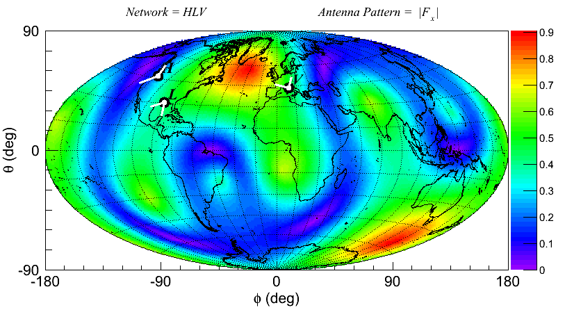
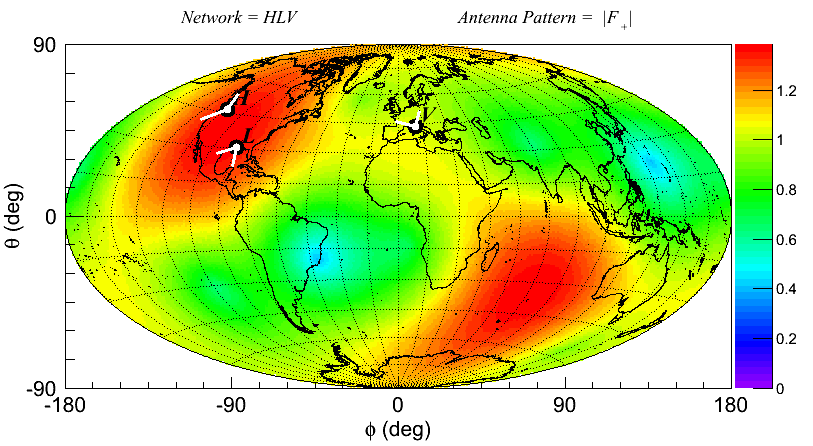
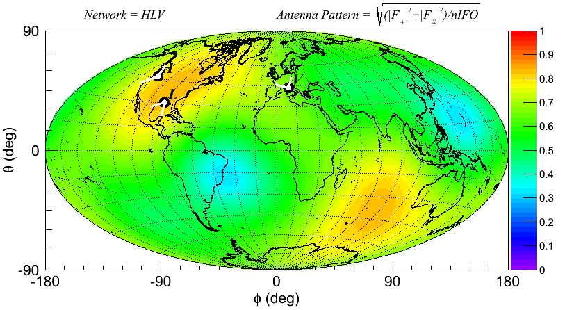
How to plot Network Antenna Pattern
Under the directory
$HOME_WAT/tools/gwat/tutorials/
there are 3 macros :
DrawAntennaPattern.C
used to plot AntPat of BuiltIn Detectors
DrawAntennaPatternUdD.C
used to plot AntPat of User Defined Detectors
DrawAntennaPatternScalar.C
used to plot AntPat of BuiltIn Detectors for Scalar GW
Examples :
* Plot |Fx| in DPF of L1H1V1 network
  - root -l 'DrawAntennaPattern.C("L1H1V1",0)'
* Plot |F+| in DPF of L1H1V1 network
  - root -l 'DrawAntennaPattern.C("L1H1V1",1)'
* Plot sqrt(|F+|^2+|Fx|^2) in DPF of L1H1V1 network
  - root -l 'DrawAntennaPattern.C("L1H1V1",3)'
* Plot |F+| in DPF of L1H2H3V1 network  (H2H3 are IFOs with V-shape : 45deg)
  - root -l DrawAntennaPatternUdD.C

* Plot sqrt(|F+|^2+|Fx|^2) in DPF of L1H1V1 network for Scalar GW
  - root -l 'DrawAntennaPatternScalar.C("L1H1V1",3)'

For more options see the macro code
How to dump the frame file contents
framelib provides some utils to manage frames.
FrDump is used to dump the frame contents.

Example :

  - FrDump -d 4 -i H-H1_LDAS_C02_L2-955609344-128.gwf

  for more options do 'FrDump -h'
How to create a celestial skymask
Look sky mask for a description of what skymask is.
to create a celestial skymask use macro
$HOME_WAT/tools/cwb/tutorials/CreateCelestialSkyMask.C
To change setup use the '#define' at the beginning of the macro code.

#define SAVE_SKYMASK            // Uncomment to save skymask file
#define SOURCE_GPS -931158395   // if SOURCE_GPS<0 then SOURCE_RA/DEC are geographic coordinates
                            // if SOURCE_GPS>0 then SOURCE_RA/DEC are celestial coordinates
#define SOURCE_RA  60       // geographic/celestial coordinate longitude/ra
#define SOURCE_DEC 30       // geographic/celestial coordinate latitude/dec
#define SKYMASK_RADIUS 20   // skymask radius in degrees centered at (SOURCE_RA,SOURCE_DEC)

To run macro do :
root -l $HOME_WAT/tools/cwb/tutorials/CreateCelestialSkyMask.C

The previous definitions produce a skymask centered to ra/dec=93.9/30 deg with radius=20 deg
If SAVE_SKYMASK is uncommented the final name file is :
CelestialSkyMask_DEC_30d0_RA_93d9_GPS_N931158395d0_RADIUS_20d0.txt
if #define DRAW_SKYMASK is uncommented macro display the following image :

How to plot skymap

How to make gw frame file list with gw_data_find
list available observatories :
gw_data_find -w --show-observatories

output is :

G
GHLTV
GHLV
H
HL
L
V
list available types :
gw_data_find -y --show-types

output is :

H1_LDAS_C00_L2
H1_LDAS_C02_L2
H1_LDAS_C02_L2_CWINJ_TOT
H1_LDR_C00_L2
H1_LDR_C02_L2
H1_NINJA2_G1000176_EARLY_GAUSSIAN
H1_NINJA2_GAUSSIAN
list gps-second segments for all data of type specified :
gw_data_find -a --show-times

gw_data_find --observatory=H --type=H1_LDAS_C02_L2 --show-times

output is :

931035328 931116384
931116544 931813504
931813664 932228288
932228896 932231584
...
list of H1 data files of type H1_LDAS_C02_L2 found in a gps range :
gw_data_find --observatory=H --type=H1_LDAS_C02_L2                    \
  --gps-start-time=955609344 --gps-end-time=955609544 --url-type=file

output is :

file://localhost/atlas/ldr/d11/H/H1_LDAS_C02_L2/0955/609000/H-H1_LDAS_C02_L2-955609344-128.gwf
file://localhost/atlas/ldr/d11/H/H1_LDAS_C02_L2/0955/609000/H-H1_LDAS_C02_L2-955609472-128.gwf

gw_data_find --observatory=GHLV --type=BRST_S6_10Q2                   \
  --gps-start-time=955609344 --gps-end-time=955609544--url-type=file

output is :

file://localhost/atlas/ldr/d11/GHLV/BRST_S6_10Q2/0955/609000/GHLV-BRST_S6_10Q2-955609215-1000.gwf
gw_data_find can be used to generate the frame list files used by cWB :
gw_data_find --observatory=H --type=H1_LDAS_C02_L2 --url-type=file    \
  --gps-start-time=955609344 --gps-end-time=955609544 > H1_LDAS_C02_L2_955609344_955609544.frl
here are reported the instructions to produce the frame lists used in the example S6A_R4_BKG_L1H1V1
gw_data_find --observatory=H --type=H1_LDAS_C02_L2 --url-type=file    \
  --gps-start-time=931035520 --gps-end-time=935798528 > input/S6A_R3_H1_LDAS_C02_L2.frames

gw_data_find --observatory=L --type=L1_LDAS_C02_L2 --url-type=file    \
  --gps-start-time=931035520 --gps-end-time=935798528 > input/S6A_R3_L1_LDAS_C02_L2.frames

gw_data_find --observatory=V --type=HrecV3 --url-type=file            \
  --gps-start-time=931035520 --gps-end-time=935798528 > input/S6A_R1_V1_HrecV3.frames
How to create data quality file list
Data quality are established from the LIGO-Virgo collaboration according to the system information from the detectors. It is necessary to apply data quality in production phase to exclude possible GW-like triggers surely due to environmental or instrumental origin.
Warning
The following instrictions refer to S6 run. Starting from O1,O2 runs cWB pipeline uses the data quality stored in the cWB config git repository.
Note
cWB pipeline uses CAT0,1,2,4 in production stage and CAT3 or HVETO in post-production stage. See How job segments are created
There are three commands:
ligolw_segment_query: extract science mode information
ligolw_segments_from_cats: extract data quality information
ligolw_print: extract time lists
To extract data quality, you should know where is the database (for
instance https://segdb.ligo.caltech.edu) and the xml file containing
the data quality definition (for instance
https://www.lsc-group.phys.uwm.edu/bursts/public/runs/s6/dqv/category_definer/)
Examples: Let’s consider the data quality used for this example: S6A_R4_BKG_L1H1V1_SLAG
We need to know:
database: https://segdb.ligo.caltech.edu
data quality definition file: https://www.lsc-group.phys.uwm.edu/bursts/public/runs/s6/dqv/category_definer/H1L1V1-S6D_BURST_ALLSKY_OFFLINE-961545615-0.xml
start, stop: 931035615, 935798415
Science mode definition: H1:DMT-SCIENCE:4, L1:DMT-SCIENCE:4, V1:ITF_SCIENCEMODE
Obtained these information we can proceed. There are three steps:
Virgo Science segment list for period
ligolw_segment_query                                                    \
  --segment-url https://segdb.ligo.caltech.edu --query-segments         \
  -d -s 931035615 -e 935798415 --include-segments V1:ITF_SCIENCEMODE |  \
  ligolw_print --table segment --column start_time --column end_time    \
  --delimiter " "> S6A_OFFLINE_V1SCIENCE.txt
To obtain the other detectors, just substitute V1:ITF_SCIENCEMODE with the other Science mode, and the name of the output file (S6A_OFFLINE_V1SCIENCE.txt)
- LIGO-Virgo data quality xml files, separating the different categories (CAT1-2-3-4).This command create some xml files in the xml directory, each one specific of one category and one detector, for instance: for Virgo CAT1:* V1-VETOTIME_CAT1-931035615-4762800.xml
ligolw_segments_from_cats                                                       \
  --veto-file=https://www.lsc-group.phys.uwm.edu/bursts/public/runs/s6/         \
  dqv/category_definer/H1L1V1-S6A_BURST_ALLSKY_OFFLINE-930960015-5011200.xml    \
  --gps-start-time=931035615  --gps-end-time=935798415 -d --separate-categories \
  --segment-url https://segdb.ligo.caltech.edu -o xml/
Get lists from xml, for instance for V1 CAT1:
ligolw_print                                                                    \
  xml/V1-VETOTIME_CAT1-931035615-4762800.xml --table segment                    \
  --colum start_time --column end_time --delimiter " "                          \
  > S6A_OFFLINE_V1_DQCAT1SEGMENTS.txt
To obtain the other detectors, just substitute detector (
V1) and category (CAT1) in input (xml/V1-VETOTIME_CAT1-931035615-4762800.xml) and output (S6A_OFFLINE_V1_DQCAT4SEGMENTS.txt) files.
How to use the Condor batch system to play with jobs
SUB FILE : condor/ADV_SIM_BRST_L1H1V1_run1.sub
Universe = vanilla
getenv = true
priority = $(PRI)
on_exit_hold = ( ExitCode != 0 )
request_memory = 3000
executable = net.sh
environment = "cWB_JOBID=$(PID)"
output = /home/waveburst/ADV_SIM_BRST_L1H1V1_run1/log/$(PID)_ADV_SIM_BRST_L1H1V1_run1.out
error = /home/waveburst/ADV_SIM_BRST_L1H1V1_run1/log/$(PID)_ADV_SIM_BRST_L1H1V1_run1.err
log = /local/user/waveburst/ADV_SIM_BRST_L1H1V1_run1.log
notification = never
rank=memory
queue
DAG FILE : condor/ADV_SIM_BRST_L1H1V1_run1.dag (1 job)
JOB A1 /home/waveburst/ADV_SIM_BRST_L1H1V1_run1/condor/ADV_SIM_BRST_L1H1V1_run1.sub
VARS A1 PID="1"
RETRY A1 3000
cd condor
condor_submit_dag ADV_SIM_BRST_L1H1V1_run1.dag
To see the job status of user waveburst do :
condor_q waveburst
To see the global user status :
condor_userprio -all
To remove a job do :
condor_rm jobid
jobdid is the first number of each line reported by the command condor_q
To hold all jobs in idle status belonging to the user waveburst do :
condor_q waveburst | grep " I " | awk '/waveburst/ {print $1}' | xargs condor_hold
To remove all jobs belonging to the user waveburst do :
condor_q waveburst | awk '/waveburst/ {print $1}' | xargs condor_rm
To release jobs with id [24086884.0:24087486.0] belonging to the user waveburst do :
condor_q waveburst | awk '$0>24086884.0' | awk '$0<24087486.0' | \
  awk '/waveburst/ {print $1}' | xargs condor_release
How to read the event’s parameters from the output root files produced by the cWB pipeline
The wave and mdc root files can be read from a macro. The following examples
ReadFileWAVE.C
ReadFileMDC.C
show how to do.
The macro :
trunk/tools/cwb/tutorials/ReadFileWAVE.C
show how to read event parameters from root wave file
The macro must be modified according what user needs.
To run the macro do :
root -l 'ReadFileWAVE.C("merge/wave_file_name.root",nIFO)'
where nIFO is the number of detectors in the network

The macro :
trunk/tools/cwb/tutorials/ReadFileMDC.C
show how to read event parameters from root mdc file
The macro must be modified according what user needs.
To run the macro do :
root -l 'ReadFileMDC.C("merge/mdc_file_name.root",nIFO)'
where nIFO is the number of detectors in the network

Both macros can be used also to read events from the single output root job files:
root -l 'ReadFileWAVE.C("output/wave_file_name_jobxxx.root",nIFO)'
root -l 'ReadFileMDC.C("output/wave_file_name_jobxxx.root",nIFO)'
ReadFileWAVE.C
ReadFileMDC.C
show how to read some parameters.
How to use the On The Fly MDC
cWB_Plugin_MDC_OTF.C
Config Plugin to generate injected on the fly EOBNRv2 from LAL : Config - :cwb_library:`cWB_Plugin_MDC_OTF_Config_EOBNRv2pseudoFourPN.C
Config Plugin to generate injected on the fly NSNS from LAL : Config - :cwb_library:`cWB_Plugin_MDC_OTF_Config_NSNS.C
Config Plugin to generate injected on the fly Burst MDC : Config - :cwb_library:`cWB_Plugin_MDC_OTF_Config_BRST.C
Config Plugin to generate injected on the fly eBBH MDC : Config - :cwb_library:`cWB_Plugin_MDC_OTF_Config_eBBH.C
The OTC Plugin and the configuration macro must be declared in the user_parameters.C file.
plugin = TMacro("cWB_Plugin_MDC_OTF.C");                    // Macro source
configPlugin = TMacro("cWB_Plugin_MDC_OTF_Config_BRST.C");  // Macro config
For a more details see : Plugins
How to use a distance distribution instead of a fixed hrss one for On The Fly MDC
The usual injection procedure (simulation=1) consists of injecting for each amplitude factors the same number of events for each waveform. In this way statistic for each hrss (n) depends on the analyzed time (T), injection rate (R) and waveforms number (N) in the following way: n = T*R/N.
Setting simulation=4 allows one to define a distance distribution to be used for injecting MDC. In this way the hrss distributions are not discrete, but continous. Given that at high amplitudes the expected efficiency approaches unity, we can modify the hrss distribution of injected wave amplitudes as to increase the statistic at low amplitude at the expense of the number of high amplitude signals.
You have to set the following things:
Expected hrss50% for each waveform: this is used to assure that the efficiency curve is complete for each waveform
Distance range (in a form of [d_min,d_max]): limits are expressed in kpc, hrss50% is linked to 10 kpc, reminding that distance*hrss=costant;
Distance distribution (using a formula);
cWB_Plugin_Sim4_BRST_Config.C
cWB_Plugin_Sim4.C
On the user_parameters.C in the Simulation parameters the settings are:
simulation = 4;
nfactor = 25;
double FACTORS[] ={...};
for(int i=0;i<nfactor;i++) factors[i]=FACTORS[i];
The variable factors[i] no longer has the same meaning as for simulation=1. Using more factors allows increasing statistics, the number of events for each waveform (n) if you consider observation time (T), waveforms number (N), injection rate (R) and nfactor (M) is now: n = (T*R/N)*M The real values of factors[i] reported in the user_parameters.C are not important, because the analysis substitute them with a progressive number.
The distance distribution is defined in the ConfigPlugin (put reference). In the library are integrated formula of the type: x*n over n could be any number. These can be defined in the way:
par.resize(4);
par[0].name="entries";par[0].value=100000;
par[1].name="rho_min";par[1].value=.2;
par[2].name="rho_max";par[2].value=60.;
par[3].name="rho_dist";par[3].value=1.;
MDC.SetSkyDistribution(MDC_RANDOM,par,seed);
where
par[0] is …;
par[1] and par[2] are minimum and maximum distance, in kpc;
par[3] is the exponent of the distribution (n)
It is also possible to set a user-defined function for distribution in this way:
par.resize(3);
par[0].name="entries";par[0].value=100000;
par[1].name="rho_min";par[1].value=.2;
par[2].name="rho_max";par[2].value=60.;
MDC.SetSkyDistribution(MDC_RANDOM,"formula",par,seed);
where the formula is of the type f(x), for instance :
MDC.SetSkyDistribution(MDC_RANDOM,"x",par,seed);
equivalent to the example above where we define the rho_dist=1 for the par[3].
How to do an interactive multistages 2G analysis
The 2G configuration setup is : config/user_parameters.C
The network is L1H1V1
The noise is a simulated gaussian noise with advanced detectors PSD
The MDC is a NSNS injection produced “On The Fly” from LAL (Injected with a network SNR=120)
Search is unmodeled rMRA
Use 6 resolution levels (from 3 to 8)

SETUP : create working directories + generate simulated noise
*The following is the list of the preliminary steps for the setup:
setup the cwb environment according to the cluster type : cWB quick startup
- copy the example directory :
cp -r $HOME_LIBS/WAT/trunk/tools/cwb/examples/ADV_SIM_NSNS_L1H1V1_MultiStages2G MultiStages2G
- change directory :
cd MultiStages2G
- - create working directories- create noise frames with simulated ADV strain
make setup
INIT STAGE : Read Config / CAT1-2 / User Plugin
 to process the INIT stage execute the command:
cwb_inet2G config/user_parameters.C INIT 1
the output root file is:data/init_931158208_192_MultiStages2G_job1.rootto display the contents of the output root file use the following commandsbrowse the root file: ( )

root data/init_931158208_192_MultiStages2G_job1.rootfrom the ROOT browser type:new TBrowserthen double click the folder ROOT files and then on the itemdata/init_931158208_192_MultiStages2G_job1.rootthe following sub items are displayed:config;1 network;1 history;1 cwb;1
to see the contents of objects double click on the specific itemNote: the config,history items are opened in the vi viewer, to exit type : and then type q- to dump the cWB config from shell command do:
cwb_dump config data/init_931158208_192_MultiStages2G_job1.root dump
the output config txt file is:report/dump/init_931158208_192_MultiStages2G_job1.Cto view with the cWB config from shell command do:cwb_dump config data/init_931158208_192_MultiStages2G_job1.root
- to dump the cWB history from shell command do:
cwb_dump history data/init_931158208_192_MultiStages2G_job1.root dump
the output history txt file is:report/dump/init_931158208_192_MultiStages2G_job1.historyto view with the cWB history from shell command do:cwb_dump history data/init_931158208_192_MultiStages2G_job1.root
STRAIN STAGE : Read gw-strain / MDC data frames(or On The Fly MDC)
 to process the STRAIN stage execute the command:
cwb_inet2G data/init_931158208_192_MultiStages2G_job1.root STRAIN
the output root file is:data/strain_931158208_192_MultiStages2G_job1.rootto display infos about strain/mdc use the following commandsproduce L1 PSD and visualize the plot in the ROOT browser ( )

cwb_inet2G data/init_931158208_192_MultiStages2G_job1.root STRAIN "" \
           '--tool psd --ifo L1 --type strain --draw true'
- produce L1 PSD and save the plot under the report/dump directory
cwb_inet2G data/init_931158208_192_MultiStages2G_job1.root STRAIN "" \
           '--tool psd --ifo L1 --type strain --draw true --save true'
the output png file is:report/dump/psd_STRAIN_L1_931158200_MultiStages2G_job1.png - display H1 noise with `FrDisplay <frdisplay.html#frdisplay>`__
cwb_inet2G data/init_931158208_192_MultiStages2G_job1.root STRAIN "" \
           '--tool frdisplay --hpf 50 --decimateby 8 --ifo H1 --type strain'
- display injected waveforms in ROOT browser (Time/FFT/TF domain)
cwb_inet2G data/init_931158208_192_MultiStages2G_job1.root STRAIN "" \
           '--tool inj --draw true'
- double click on L1 folder, select the item L1:50.00;1 and open the popup menu with the right mouse bottomThe following options are available :- PlotTime : Plot waveform in time domain ( )

PlotFFT : Plot waveform FFT ( )

PlotTF : Plot waveform spectrogram ( )
 - PrintParameters : Show waveform infos (start,stop,rate,…)- PrintComment : Show the MDC log file infos (MDC type, start, ifos, antenna pattern, …)- DumpToFile : Dump waveform to ascii file
CSTRAIN STAGE : Data Conditioning (Line Removal & Whitening)
 to process the CSTRAIN stage execute the command:
cwb_inet2G data/init_931158208_192_MultiStages2G_job1.root CSTRAIN
the output root file is:data/strain_931158208_192_MultiStages2G_job1.rootto display infos about noise use the following commandsproduce L1 nRMS estimated at GPS=931158300.55 and and save it to a file
cwb_inet2G data/init_931158208_192_MultiStages2G_job1.root CSTRAIN "" \
           '--tool nrms --ifo L1 --type strain --gps 931158300.55'
the output txt file is:report/dump/nrms_gps931158300.55_STRAIN_L1_931158200_MultiStages2G_job1.txtproduce L1 T/F nRMS and visualize the plot in the ROOT browser ( )

cwb_inet2G data/strain_931158208_192_MultiStages2G_job1.root CSTRAIN "" \
           '--tool nrms --ifo L1 --type strain --draw true'
- produce whitened H1 PSD and visualize the plot in the ROOT browser
cwb_inet2G data/strain_931158208_192_MultiStages2G_job1.root CSTRAIN "" \
           '--tool psd --ifo H1 --type white --draw true'
- produce whitened H1 PSD and save the plot under the report/dump directory
cwb_inet2G data/strain_931158208_192_MultiStages2G_job1.root CSTRAIN "" \
           '--tool psd --ifo H1 --type white --draw true --save true'
the output png file is:report/dump/psd_WHITE_H1_931158200_MultiStages2G_job1.pngto display the output png file do:display report/dump/psd_WHITE_H1_931158200_MultiStages2G_job1.png - produce whitened H1 TF WDM and visualize the plot in the ROOT browser
cwb_inet2G data/strain_931158208_192_MultiStages2G_job1.root CSTRAIN "" \
           '--tool wdm --ifo L1 --type white --draw true'
- double click on L1:level-8;1 folderThere are three type of plots:- L1:tf:white-8;1 - scalogram of whitened L1 data at resolution level=8 ( )

L1:t:white-8;1 - projection on time axis of scalogram of whitened L1 data at resolution level=8 ( )

L1:f:white-8;1 - projection on frequency axis of scalogram of whitened L1 data at resolution level=8 ( )

COHERENCE STAGE : TF Pixels Selection
 to process the COHERENCE stage execute the command:
cwb_inet2G data/cstrain_931158208_192_MultiStages2G_job1.root COHERENCE
the output root file is:data/cstrain_931158208_192_MultiStages2G_job1.rootto display infos about data processed in this stage use the following commands- produce TF WDM of maximum energy (before the pixel selection) at level 8 and visualize the plot in the ROOT browser
cwb_inet2G data/cstrain_931158208_192_MultiStages2G_job1.root COHERENCE "" \
           '--tool emax --level 8  --draw true'
In the browser are listed 4 folders : L1,H1,V1,NET - NET folder is the sum of 3 detectors max energyFor each folder there are three type of plots (Ex:NET):- L1:tf:0-8;1 - scalogram of NET max energy at resolution level=8 and factor=0 ( ) - L1:t:0-8;1 - proj on time axis of NET max energy at resolution level=8 and factor=0- L1:f:0-8;1 - proj on frequency axis of NET max energy at resolution level=8 and factor=0
SUPERCLUSTER STAGE : Clustering & Cluster Selection
 to process the SUPERCLUSTER stage execute the command:
cwb_inet2G data/coherence_931158208_192_MultiStages2G_job1.root SUPERCLUSTER
the output root file is the trigger file:data/supercluster_931158208_192_MultiStages2G_job1.rootto display the contents of the trigger file use the following commandsbrowse the root file: ( )

root data/supercluster_931158208_192_MultiStages2G_job1.rootfrom the ROOT browser type:new TBrowserthen double click the folder ROOT files and then on the itemdata/supercluster_931158208_192_MultiStages2G_job1.rootthe following sub items are displayed:config;1 network;1 history;1 cwb;1 sparse - contains the sparse maps supercluster - contains the cluster structures waveform - contains the whitened injected waveforms
to see the contents of objects double click on the specific item- produce TF WDM of L1 sparse map and visualize the plot in the ROOT browser
rm data/wave_931158208_192_MultiStages2G_120_job1.root

cwb_inet2G data/coherence_931158208_192_MultiStages2G_job1.root SUPERCLUSTER "" \
           '--tool sparse --type supercluster --ifo L1 --draw true'
From the ROOT browser double click the folder L1:level-8;1 and double click on L1:tf:sparse;8;1The plot show the L1 scalogram of the sparse map at resolution level=8 ( )
In the sparse map are displayed the core pixels & the halo pixels. See the `SSeries :cwb_library:`SSeries` class
LIKELIHOOD STAGE : Event Reconstruction & Output Parameters
 to process the LIKELIHOOD stage execute the command:
cwb_inet2G data/supercluster_931158208_192_MultiStages2G_job1.root LIKELIHOOD
the output root file is:data/wave_931158208_192_MultiStages2G_job1.rootto display infos about data processed in this stage use the following commands- produce CED of the event
cwb_inet2G data/supercluster_931158208_192_MultiStages2G_job1.root LIKELIHOOD "" ced
the output CED is:ced_931158208_192_MultiStages2G_60_job1To browse the ced data from web the directory must be moved to report/ced :mv ced_931158208_192_MultiStages2G_60_job1 report/ced/
The web link in ATLAS is : https://ldas-jobs.ligo.caltech.edu/~username/LSC/reports/MultiStages2G
- produce TF WDM of L1 sparse map and visualize the plot in the ROOT browser
rm data/wave_931158208_192_MultiStages2G_120_job1.root

cwb_inet2G data/supercluster_931158208_192_MultiStages2G_job1.root LIKELIHOOD "" \
           '--tool sparse --type likelihood --ifo L1 --draw true'
From the ROOT browser double click the folder L1:level-8;1 and double click on L1:tf:sparse;8;1The plot show the L1 scalogram of the sparse map at resolution level=8 ( )In the sparse map are displayed the core pixels & the halo pixels. See the `SSeries :cwb_library:`SSeries` class browse the root file: ( )
 If the output wave file has been removed regenerate it again :cwb_inet2G data/supercluster_931158208_192_MultiStages2G_job1.root LIKELIHOOD
root data/wave_931158208_192_MultiStages2G_120_job1.rootfrom the ROOT browser type:new TBrowserthen double click the folder ROOT files and then on the itemdata/wave_931158208_192_MultiStages2G_120_job1.rootthe following sub items are displayed:history;1 - is the history livetime - is the tree of the livetimes waveburst - is the tree of the reconstructed events mdc - is the tree of the injections
to see the contents of objects double click on the specific item- to dump the event to screen from shell command do:
cwb_dump events data/init_931158208_192_MultiStages2G_120_job1.root
- to dump the event to file from shell command do:
cwb_dump events data/wave_931158208_192_MultiStages2G_120_job1.root > \
                data/wave_931158208_192_MultiStages2G_120_job1.txt
The ascii file contains all the event reconstructed parameters
nevent:     1
ndim:       3
run:        1
rho:        52.779896
netCC:      0.963956
netED:      0.005008
penalty:    0.995367
gnet:       0.852102
anet:       0.673093
inet:       0.552534
likelihood: 1.001513e+04
ecor:       5.570363e+03
ECOR:       5.570363e+03
factor:     120.000000
range:      0.000000
mchirp:     1.218770
norm:       0.948450
usize:      0
ifo:        L1 H1 V1
eventID:    1 0
rho:        52.779896 51.804337
type:       1 1
rate:       0 0 0
volume:     2123 2123 2123
size:       48 2001 0
lag:        0.000000 0.000000 0.000000
slag:       0.000000 0.000000 0.000000
phi:        6.428571 11.458068 39.961182 6.428571
theta:      44.610798 44.999981 45.389202 44.610798
psi:        1.061384 162.416916
iota:       0.079406 0.155110
bp:          0.0198  0.2747 -0.8358
inj_bp:     -0.0083  0.2853 -0.7636
bx:          0.4046 -0.3521 -0.5458
inj_bx:      0.3606 -0.2905 -0.6452
chirp:      1.218770 1.196272 0.040930 99.997925 0.892147 0.942552
range:      0.000000 1.666667
Deff:       14.044416 8.113791 8.414166
mass:       1.400000 1.400000
spin:       0.000000 0.000000 0.000000 0.000000 0.000000 0.000000
eBBH:       0.000000 0.000000 0.000000
null:       9.100333e+01 7.176315e+01 4.972414e+01
strain:     2.857830e-22 2.435557e+01
hrss:       1.050772e-22 1.937086e-22 1.819552e-22
inj_hrss:   1.565444e-22 2.709419e-22 2.611956e-22
noise:      2.631055e-24 2.687038e-24 3.527480e-24
segment:    931158200.0000 931158408.0000 931158200.0000 931158408.0000 931158200.0000 931158408.0000
start:      931158282.0000 931158282.0000 931158282.0000
time:       931158295.7714 931158295.7725 931158295.7562
stop:       931158299.9609 931158299.9609 931158299.9609
inj_time:   931158292.0315 931158292.0323 931158292.0152
left:       82.000000 82.000000 82.000000
right:      108.039062 108.039062 108.039062
duration:   17.960938 17.960938 17.960938
frequency:  108.255516 108.255516 108.255516
low:        45.000000 45.000000 45.000000
high:       480.000000 480.000000 480.000000
bandwidth:  435.000000 435.000000 435.000000
snr:        1.819248e+03 5.394480e+03 2.919318e+03
xSNR:       1.741324e+03 5.443648e+03 2.887045e+03
sSNR:       1.666738e+03 5.493264e+03 2.855128e+03
iSNR:       2571.384766 7439.704590 3851.914307
oSNR:       1666.737793 5493.264160 2855.128418
ioSNR:      1659.589111 5176.358887 2728.931152
netcc:      0.963956 0.872941 0.912740 0.977282
neted:      27.897186 27.897186 156.118530 212.490631 120253.312500
erA:         4.173  0.648  0.916  1.122  1.296  1.449  1.587  1.774  2.049  2.467  0.052
How to do the Parameter Estimation Analysis
cWB_Plugin_PE.C
Reconstructed waveform : median and 50,90 percentiles
Reconstructed instantaneous frequency (with Hilbert tranforms) : median and 50,90 percentiles
Reconstructed waveform vs Injected waveform (only in simulation mode)
Median SkyMap Localization
Chirp Mass and Error estimation
The following scheme shows the method :

CONFIGURATION PARAMETERS : description of the parameters used to configure the PE analysis
pe_id
    // process only ID=PE_ID [0(def) -> ALL]

pe_trials
    // number of trials (def=100)

pe_signal
    // signal used for trials : 0(def)/1/2
    // 0 - reconstructed waveform
    // 1 - injected waveform (available only in simulation mode)
    // 2 - original waveform = (reconstructed+null)

pe_noise
    // noise used for trials :  0/1(def)/2
    // 0 - waveform is injected in the whitened HoT and apply
               Coherent+SuperCluster+Likelihood stages
    // 1 - add gaussian noise to likelihood sparse maps and apply Likelihood stage
    // 2 - add whitened HoT to likelihood sparse maps and apply Likelihood stage

pe_amp_cal_err
    // max percentage of amplitude miscalibration : def(0) -> disabled
    // if>0 -> uniform in [1-pe_amp_cal_err,1+pe_amp_cal_err] else gaus(1,pe_amp_cal_err)
           Example :
             pe_amp_cal_err=0.1  // det1 : amp miscal         (uniform in -0.9,+1.1)
             pe_amp_cal_err=0.1  // det2 : ...

pe_phs_cal_err
    // max phase (degrees) miscalibration : def(0) -> disabled
    // if>0 -> uniform in [-pe_phs_cal_err,+pe_phs_cal_err] else gaus(pe_phs_cal_err)
           Example :
             pe_phs_cal_err=10   // det1 : phase miscal (deg) (uniform in -10,+10)
             pe_phs_cal_err=10   // det2 : ...

pe_multitask
    // true/false(def)
           if enabled, PE trials are executed by different jobs in multitask
           only simulation=0 and single event (gps>0)

pe_ced_dump
    // dump CED at gLRETRY=PE_CED_DUMP (def(-1) -> disabled)

pe_skymask
    // skymask used for trials : 0(def)/1/2/3
    // 0 - disable -> search over all sky
    // 1 - skymask with radius 0.1(deg) and source selected according
               the reconstructed skymap probability
    // 2 - skymask select only the sky position where the waveform
               is reconstructed (the maximum of detection statistic)
    // 3 - skymask select only the sky position where the waveform
               has been injected

pe_seed
    // seed used by PE for random generation - 0(def) -> random seed


pe_gps
    // if >0 only gps +/- iwindow is analyzed - 0(def) -> disabled
           Example : pe_gps=1167554561


pe_ced options
        // the following options are available : tfmap/rdr/skymap/rec/inj/rinj/cm/distr/null
           Example : to enable/disable tfmap do : pe_ced_tfmap_enable/pe_ced_tfmap_disable

        // tfmap   - pe_ced_enable(def)/disable
           Shows/Hides the Time-Frequency Maps Tab -> Spectrograms, Scalograms, TF Likelihood,Null

    // rdr     - pe_ced_enable(def)/disable
           Shows/Hides Reconstructed Detector Response Tab

    // skymap  - pe_ced_enable(def)/disable
           Shows/Hides SkyMaps Tab

    // rec     - pe_ced_enable(def)/disable
           Shows/Hides Reconstructed Waveforms/Instantaneous-Frequency with errors Tab

    // inj     - pe_ced_enable(def)/disable
           Shows/Hides the Injection tab reporting the comparison with the injected whitened waveform

    // rinj    - pe_ced_enable/disable(def)
           Shows/Hides the Injection tab reporting the comparison with the injected whitened waveform
       in the time-frequency subspace of the PointEstimated waveform

    // cm      - pe_ced_enable(def)/disable
           Shows/Hides Chirp Mass Value/Error Distributions Tab

    // distr   - pe_ced_enable/disable(def)
           Shows/Hides Residuals Distributions Tab

    // null    - pe_ced_enable/disable(def)
           Shows/Hides Null Pixels Distributions Tab

    // pca     - pe_ced_enable/disable(def)
           Shows/Hides the PCA TF likelihood to the tfmap Tab
           Note : tfmap must be enabled

pe_output options
        // dump objects on the output wave root file (only if cedDump=false)
        // by default all are disabled
        // Example : to enable/disable reconstructed waveform
                     pe_output_enable=rec  / pe_output_disable=rec
        // options
           inj    // save injection to the output root file
           rec    // save reconstructed waveform to the output root file
           wht    // save whitened data (inthe time range of rec) to the output root file
           med    // save median to the output root file
           p50    // save percentile 50 to the output root file
           p90    // save percentile 90 to the output root file
           avr    // save averaged waveform to the output root file
           rms    // save RMS to the output root file
SETUP : how to setup the PE
The PE parameter must be defined in the user_parameters.C file :
- define the plugin
plugin = TMacro(gSystem->ExpandPathName("$HOME_cWB/plugins/cWB_Plugin_PE.C"));
if you need to compile the plugin then copy the plugin into your working folder in macro directory :
cp $HOME_cWB/plugins/cWB_Plugin_PE.C macro/.
compile :
root -l -b macro/cWB_Plugin_PE.C++
add the following lines in the user_parameters.C file :
plugin = TMacro("macro/cWB_Plugin_PE.C");
plugin.SetTitle("macro/cWB_Plugin_PE_C.so");
- Add PE parameters (this is an example) :
cedDump=true;                       // this option enable the creation of the PE CED
                                       it is an extended version of the standard CED
                                       Note : if cedDump is enabled then the pe_output option
                                              are disabled
                                              pe_output enable output on wave root file
                                              which is not produced when CED is enabled

TString optpe = "";                 // Note : add space at the end of each line
optpe += "pe_trials=100 ";           // number of trials
optpe += "pe_id=0 ";                // process all detected events
//optpe += "pe_gps=1167554561 ";      // only gps +/- iwindow is analyzed
optpe += "pe_noise=0 ";             // signal used for trials is the reconstructed
optpe += "pe_signal=0 ";            // waveform is injected in the whitened HoT and
                                    // apply for each trial Coherent+SuperCluster+Likelihood
optpe += "pe_amp_cal_err=0.1 ";     // det1 : amp miscal         (uniform in -0.9,+1.1)
optpe += "pe_phs_cal_err=10 ";      // det1 : phase miscal (deg) (uniform in -10,+10)
optpe += "pe_amp_cal_err=0.1 ";     // det2 : ...
optpe += "pe_phs_cal_err=10 ";      // det2 : ...
optpe += "pe_ced_dump=-1 ";         // dump CED at gLRETRY=PE_CED_DUMP
optpe += "pe_skymask=0 ";           // disable -> search over all sky

//optpe += "pe_multitask=true ";    // enable/disable multitask

                                    // CED options (only if cedDump=true)
optpe += "pe_ced_enable=tfmap ";
optpe += "pe_ced_enable=rdr ";
optpe += "pe_ced_enable=skymap ";
optpe += "pe_ced_enable=rec ";
optpe += "pe_ced_enable=inj ";
optpe += "pe_ced_disable=rinj ";
optpe += "pe_ced_enable=cm ";
optpe += "pe_ced_enable=distr ";
optpe += "pe_ced_enable=null ";
optpe += "pe_ced_disable=pca ";

                                    // OUTPUT options (only if cedDump=false)
optpe += "pe_output_enable=inj ";   // save injection to the output root file
optpe += "pe_output_enable=rec ";   // save reconstructed waveform to the output root file
optpe += "pe_output_enable=wht ";   // save whitened data to the output root file
optpe += "pe_output_enable=med ";   // save median to the output root file
optpe += "pe_output_enable=p50 ";   // save percentile 50 to the output root file
optpe += "pe_output_enable=p90 ";   // save percentile 90 to the output root file
optpe += "pe_output_enable=avr ";   // save averaged waveform to the output root file
optpe += "pe_output_enable=rms ";   // save RMS to the output root file

strcpy(parPlugin,optpe.Data());     // set PE plugin parameters
strcpy(comment,"pe configuration example");
RUNNING : How to run PE analysis
The PE can be executed in different modesPE on one zero lag event (simulation=0)
Note : simulation parameter must be 0single taskadd the gps parameter to the PE configuration list , for example : optpe += "pe_gps=1167554561 "; // only gps +/- iwindow is analyzed then execute the following command (consider job=40) : cwb_inet 40 0 ced // CED is produced cwb_inet 40 // CED is not produced if you want to execute in batch mode, create the dag file and select only the job 40 and do submit : cwb_condor submit condor/file.dag
multi taskin multitask mode it is possible to execute each trial with a separate job this speeds up the execution First of all we must generate a special dag file (consider job=40) The following 2 PE parameters must be declared in the user_parameters.C file : optpe += "pe_multitask=true "; optpe += "pe_trials=100 "; then execute : cwb_condor mtpe 40 Note : to output CED add cedDump=true; to user_parameters.C the following files are created under the condor directory : condor/work_dir.mtpe.sub condor/work_dir.mtpe.dag The dag file contains 100 entries, the last job is executed as last job and collect all data produced by the first 99 jobs Execute : cwb_condor submit condor/work_dir.mtpe.dag
PE with simulated injections (simulation=4)
Note : simulation parameter must be 4Note : only 1 injection per segment must be used because the PE uses the segment noise for trialsTo increase the number of injection per segment we use simulation=4 and inject 1 waveform per factorFor example, in user_parameters.C the following parameters must be declared :simulation = 4; // factors are used as a trial factor nfactor = 10; // number of factors -> 1 injection per factor factors[0]=1; // starting factor
In this operative mode we must merge the cWB_Plugin_PE.C with the Injection plugin : cWB_Plugin_MDC_OTF.Ccwb_mplugin macro/cWB_Plugin_MDC_OTF_PE.C \ $HOME_cWB/plugins/cWB_Plugin_MDC_OTF.C $HOME_cWB/plugins/cWB_Plugin_PE.C
moreover a configuration plugin must be provided and the following declarations must be added :
plugin = TMacro("macro/cWB_Plugin_MDC_OTF_PE.C");            // Macro source
configPlugin = TMacro("macro/cWB_Plugin_MDC_OTF_Config.C");  // Macro config
single taskExecute the following command (consider job=40) : cwb_inet 40 0 ced // CED is produced cwb_inet 40 // CED is not produced Note : to be sure that CED is not produced use the second option and set cedDump=false; in user_parameters.C Note : the single task mode can be used with standard condor submit procedure
multi taskin multitask mode it is possible to execute each factor with a separate job this speeds up the execution First of all we must generate a special dag file (consider job=40) Execute : cwb_condor mtpe 40 Note : to output CED add cedDump=true; to user_parameters.C the following files are created under the condor directory : condor/work_dir.mtpe.sub condor/work_dir.mtpe.dag The dag file contains nfactor entries Execute : cwb_condor submit condor/work_dir.mtpe.dag
SKYMAP STATISTIC : How to produce standard GraceDB skymaps
It is possible to include in the CED the standard skymap statistic produced for GraceDBPE produce 2 skymaps under the CED directory :skyprobcc.fits : point estimate skymap
mskyprobcc.fits : median skymap
To produce the skymaps execute the cwb_report command :
* cwb_report skymap ced_dir/skyprobcc.fits
  create the web page for skymap-statistics (point estimate) : ced_dir/skyprobcc

  The symbolic index file is copied to ced_dir and
  the link to skymap-statistics is added (Skymap Statistic ( point estimate ))
To create the skymap statistic of mskyprobcc.fits and for the comparisonbetween skyprobcc.fits and mskyprobcc.fits see the cwb_report skymap command options.
How to do a 2 stages 2G analysis in batch mode
- First Stage : ETGThe generation of the first stage is based on the standard procedure described in the first two sections PRE-PRODUCTION : Setup analysis and PRODUCTION - Run the analysis reported in the link Background ExampleThe only difference is in - Create Condor jobs.Instead of the command :
cwb_condor createuses the command :
cwb_condor create SUPERCLUSTER
The SUPERCLUSTER option forces the analysis to process data until the SUPERCLUSTER stage.The trigger files are saved under the output directory with namessupercluster_*_job#.rootIt is possible to save the trigger files in the nodes user directory and the links to these files are created under the output directory. This option allows saving local space and optimizing the I/O, but on the contrary the user node disk does not guarantee a safe place where to store the files. Use this option only if the trigger files are very largeTo force the trigger files to be saved in the nodes add this option to the config/user_parameters.C :jobfOptions|=cWB_JOBF_SAVE_NODE;
- Second Stage : RECONSTRUCTIONTo process the second stage it is necessary to create a new working directory.This directory must be a clone of the first stage directory.The command to be used to create a clone directory is cwb_clonedirHere are the instructions :
cwb_clonedir SRC_DIR_FIRST_STAGE DEST_DIR_SECOND_STAGE '--output links'
If DEST_DIR_SECOND_STAGE already exists, only links are updated
A new directory named DEST_DIR_SECOND_STAGE is created with the same input,config,macros files.The option output links forces the creation under the output dir of the links of the trigger files produced in the first stage.To create the condor files used by the second stage the following command must be used :cwb_condor recovery LIKELIHOOD
This command creates a dag file :condor/XXX.dag.recovery.xTo setup the reconstruction stage modify the config/user_parameters.CTo submit the second stages jobs do :cwb_condor submit condor/XXX.dag.recovery.x
The final output event parameter files are saved under the output directory with nameswave_*_job#.rootThe post-production is based on the standard procedure described in the last section POST-PRODUCTION : Collection of results reported in the link Background Example - Full Stage & Trigger FilesIt is possible to create the trigger files also in Full Stage analysis mode.The trigger files can be used as input for the Second Stage analysis, see Second Stage : RECONSTRUCTION.Here are the instructions :Add the following option to the user_parameters.C file :
jobfOptions|=cWB_JOBF_SAVE_TRGFILE;
Create and Submit the condor jobs.
cwb_condor create
cwb_condor submit
wave*.root and supercluster*.root files are created under the output directory.
How to merge multiple backgrounds into a single report
cwb_clonedir src_dir_1 dest_dir '--output merge'

         The src_dir_1 is cloned to dest_dir
         Search the max merged version in the src dir
         and merge wave&live tree under the dest output dir

cwb_clonedir src_dir_2 dest_dir '--output merge --config check'

         The src_dir_2 is not cloned to dest_dir because dest_dir already exists
         Search the max merged version in the src dir
         and merge wave&live tree under the dest output dir

         the option '--config check ' is used to force
         the control of compatibility of src and dest config.
         The diff is generated and user must decide if the configurations are compatible.
         If the answer is 'n' the operation is aborted.

cd dest_dir

cwb_merge M1

         all src merged files are merged into a single file under the merge directory


At this stage it is possible to apply the standard post-production procedures

the super-report

         It is possible to add to the final report the reports produced for src_dir_1 and src_dir_2 analysis.
         In the final report each report is shown as a tab entry in a tabbed html page
         This can be done using the post parameter string array pp_sreport and must be declared
         in the user_pparameters.C file.

         The syntax is :

         pp_sreport[0] = "--links http_link_to_report_1 --label label_report_1"
         ...
         pp_sreport[n] = "--links http_link_to_report_n --label label_report_n"

         where :
         - http_link_to_report_n is the http link to the report n
         - label_report_n        is the label reported in the tab


NOTE : there are some operations that can not be done.
       1 - Job statistic is not computed in the report page
       2 - CEDs can not be generated
       these quantities must be evaluated in the original src_dir
How to do the analysis of the most significant events
- Create the dag file


  We use the command cwb_report with the option loudest


  cwb_report merge_label loudest '--odir loudest_dir --rho 7 --ufile xuser_parameters.C --veto true --nevt 10'

         merge_label        : is the merge label, for example : M1.C_cc2_gt_0d45.V_hvetoLH_cat3LH
         loudest_dir        : is the output directory were the final root files are stored
         xuser_parameters.C : is the new user parameters file
                              (same syntax used for the config/user_parameters.C)
         --rho 7            : select only events with rho[X]>7.
                              X is the value of the parameter pp_irho defined in the user_pparameters.C
         --veto true        : the post production vetoes are applied (see config/user_pparameters.C)
         --nevt 10          : only the first 10 events with rho[X]>7 are selected

  The previous command produce a dag file work_dir_label.dag.loudest.x under the condor directory.


- Submit the dag file


  cwb_condor submit work_dir_label.dag.loudest.x

  The output root files are created under the directory "loudest_dir" in the report directory

  (report/postprod/XXX/loudest_dir), where XXX is the standard post production directory


At this stage it is possible to apply the standard post production procedures. For example :


- Merge the output root files


  cwb_merge M1 '--idir report/postprod/XXX/loudest_dir --utag user_merge_tag'

         --idir : is the directory where the ouput loudest root file are stored
         --utag : is the user tag added after *.Mx -> *.Mx.U_utag

  the previous command creates a merge file under the standard merging directory.

- Apply vetoes


  If required it is possible to apply the post production vetoes using cwb_setveto


- Create report


  As final step the user can produce the final standard report using a new user_pparameters.C file :


  cwb_report loudest_merge_label create xuser_parameters.C

         loudest_merge_label : is the label of the merged loudest events
         xuser_pparameters.C : is the new user parameters file
                               (same syntax used for the config/user_pparameters.C)
How to apply a time shift to the input MDC and noise frame files
- time shift of noise dataThe parameter used to shift the noise data is an array of double :it must be declared in the user_parameters.C file.The index of the array represents the IFO index and the values are theshifts in sec that must be applied to the corresponding detector.
Example (L1,H1,V2) :
dataShift[0] = 1000;    // shift +1000 sec the L1 detector
dataShift[1] = -100;    // shift -100  sec the H1 detector
dataShift[2] = 0;       // shift 0     sec the V1 detector
- time shift of MDC dataThe parameter used to shift the MDC data is :and it must be declared in the user_parameters.C file.
The mdc_shift is a structure defined in cWB::Toolbox :
mdc_shift.startMDC
mdc_shift.stopMDC
mdc_shift.offset
The parameters startMDC,stopMDC are used to define the period in MDC data that we want to reuse for the injections.This period must exist in the MDC frame files.If mdc_shift.startMDC < 0 the mdc_shift.startMDC,mdc_shift.stopMDC are the begin,end GPS times of the input MDC frame files.
The effect of this parameter is the production of infinite replicas of the period [startMDC,stopMDC] starting from the GPS=mdc_shift.offset.// // startMDC stopMDC // ^ ^ // ................|xxxxxx P xxxxxx|.............. // // the period P is replicated starting from the offset // // offset // ^ // ...|xxxxxx P xxxxxx|xxxxxx P xxxxxx|xxxxxx P xxxxxx|... //
Example :
  mdc_shift.startMDC  = 1000
  mdc_shift.stopMDC   = 2000
  mdc_shift.offset    = 500

//                 1000            2000
//                 ^               ^
// ................|xxxxxx P xxxxxx|..............
//
// the period P is replicated starting from the offset
//
//    500             1000            2000            3000
//    ^               ^               ^               ^
// ...|xxxxxx P xxxxxx|xxxxxx P xxxxxx|xxxxxx P xxxxxx|...
//
Troubleshooting
Problem with my first cWB pipeline example
Check the following items:
if cWB is used with pre-installed libraries check setting cWB quick startup.
- check if the cWB configuration script is defined in the shell login script
example : source /home/waveburst/SOFT/WAT/trunk/waveburst_watenv.csh
- check the cWB environment variables defined in in cWB configuration file
example : setenv HOME_WAT “${HOME_LIBS}/WAT/trunk”
- check if cwb_rootrc has been copied under $HOME directory
example : cp /home/waveburst/SOFT/WAT/trunk/tools/cwb/cwb.rootrc ~/.rootrc
Theory
What is the cWB coordinate system
cWB Coordinate System

theta : [0:180] degrees
- theta=0   : North Pole
- theta=180 : South Pole

phi : [0:360] degrees
- phi=0     : Greenwich meridian
- phi increases in the east direction
It is related to the Geographic system by the following transformations (see CwbToGeographic,GeographicToCwb defined in skycoord.hh):
- theta_geo = 90-theta_cwb
-   phi_geo = phi_cwb     when phi_cwb<=180
-   phi_geo = phi_cwb-360 when phi_cwb>180
What is HEALPix
To install HEALPix see :
It is used by cWB to creates a sky map segmentation
To enable this option set in config/user/parameters.C
healpix=order;
where order is a number > 0
if order=0 then cWB uses the builtin sky segmentation.

The number of pixels is given by:

npixels(order) = 12*pow(4,order)

for example :
npixels(0) = 12
npixels(1) = 48
npixels(2) = 192
npixels(3) = 768
npixels(4) = 3072
npixels(5) = 12288
npixels(6) = 49152
npixels(7) = 196608
npixels(8) = 786432


What are lags and how to use them
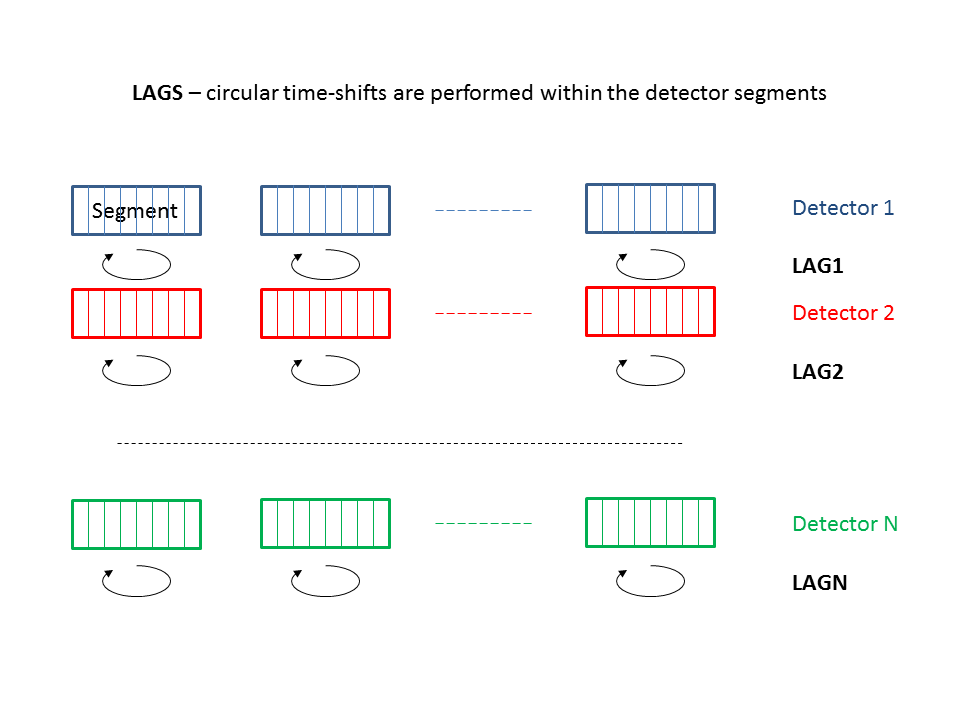
To assess the significance of a burst candidate event, we need to know the statistical properties of the background of transient accidentals. Given the intrinsic non stationarity of our data and the large deviations of any of our test statistics wrt any known statistical distribution, we are forced to empirically estimate such distributions. To resample our data set we use the well-known standard technique of the time shifted analysis.
The cWB pipeline applies relative time shifts to the detectors data streams and for each set of time lags (one per detector) a complete analysis is performed. The ensemble of these time-lagged analyses (properly rescaled by each live time) are combined to produce the False Alarm Distribution as a function of the rho. To do so, cWB divides the total observation time into time segments, with variable length between segMLS and segLen (typically between 300 and 600 s). For each segment, a job is sent to the computing cluster: within the job, cWB performs both the time-lagged analyses (i.e. by applying shifts in circular buffers) and the zero-lag analysis at the same time without increasing too much the computational load. We typically produce 200 time-lagged analyses + the zero lag.
This approach produces a “local” estimate of the accidental background, i.e. estimated within each segment. As a consequence, the number of useful time slides is limited by the minimum time shift step, O(1s), due to detectors autocorrelation and minimal length of the segments, segMLS (other than by the number of available detectors).
To perform a time-lagged analysis we have two main choices:
- the built-in lags;
the user has to set:
lagSize : number of lags
lagOff : first lag id in the list
lagStep : time step (ts)
lagMax : maximum time lag (Tm)
Applied shifts Tk are multiples of time step ts: Tk = k*ts (k is an integer).
- provide a custom set of lags via an ascii file
The parameter lagStep is not used, instead two more parameters must be used:
the ascii file name : lagFile
the lag mode to “read”: lagMode[0] = ‘r’;
A detailed description of the lag configuration parameters can be found in Production parameters.
An example of a custom lags ascii file content for a network of 3 detectors
0 0   0   0
1   0   1   200
2   0   200 1
3   0   3   198
4   0   198 3
5   0   5   196
6   0   196 5
7   0   7   194
8   0   194 7
9   0   9   192
10  0   192 9
11  0   11  190
12  0   190 11
13  0   13  188
14  0   188 13
15  0   15  186
16  0   186 15
17  0   17  184
18  0   184 17
19  0   19  182
20  0   182 19
21  0   21  180
22  0   180 21
23  0   23  178
24  0   178 23
25  0   25  176
26  0   176 25
27  0   27  174
28  0   174 27
29  0   29  172
30  0   172 29
31  0   31  170
32  0   170 31
33  0   33  168
34  0   168 33
35  0   35  166
36  0   166 35
37  0   37  164
38  0   164 37
39  0   39  162
40  0   162 39
41  0   41  160
42  0   160 41
43  0   43  158
44  0   158 43
45  0   45  156
46  0   156 45
47  0   47  154
48  0   154 47
49  0   49  152
50  0   152 49
51  0   51  150
52  0   150 51
53  0   53  148
54  0   148 53
55  0   55  146
56  0   146 55
57  0   57  144
58  0   144 57
59  0   59  142
60  0   142 59
61  0   61  140
62  0   140 61
63  0   63  138
64  0   138 63
65  0   65  136
66  0   136 65
67  0   67  134
68  0   134 67
69  0   69  132
70  0   132 69
71  0   71  130
72  0   130 71
73  0   73  128
74  0   128 73
75  0   75  126
76  0   126 75
77  0   77  124
78  0   124 77
79  0   79  122
80  0   122 79
81  0   81  120
82  0   120 81
83  0   83  118
84  0   118 83
85  0   85  116
86  0   116 85
87  0   87  114
88  0   114 87
89  0   89  112
90  0   112 89
91  0   91  110
92  0   110 91
93  0   93  108
94  0   108 93
95  0   95  106
96  0   106 95
97  0   97  104
98  0   104 97
99  0   99  102
100 0   102 99
101 0   101 100
102 0   100 101
103 0   103 98
104 0   98  103
105 0   105 96
106 0   96  105
107 0   107 94
108 0   94  107
109 0   109 92
110 0   92  109
111 0   111 90
112 0   90  111
113 0   113 88
114 0   88  113
115 0   115 86
116 0   86  115
117 0   117 84
118 0   84  117
119 0   119 82
120 0   82  119
121 0   121 80
122 0   80  121
123 0   123 78
124 0   78  123
125 0   125 76
126 0   76  125
127 0   127 74
128 0   74  127
129 0   129 72
130 0   72  129
131 0   131 70
132 0   70  131
133 0   133 68
134 0   68  133
135 0   135 66
136 0   66  135
137 0   137 64
138 0   64  137
139 0   139 62
140 0   62  139
141 0   141 60
142 0   60  141
143 0   143 58
144 0   58  143
145 0   145 56
146 0   56  145
147 0   147 54
148 0   54  147
149 0   149 52
150 0   52  149
151 0   151 50
152 0   50  151
153 0   153 48
154 0   48  153
155 0   155 46
156 0   46  155
157 0   157 44
158 0   44  157
159 0   159 42
160 0   42  159
161 0   161 40
162 0   40  161
163 0   163 38
164 0   38  163
165 0   165 36
166 0   36  165
167 0   167 34
168 0   34  167
169 0   169 32
170 0   32  169
171 0   171 30
172 0   30  171
173 0   173 28
174 0   28  173
175 0   175 26
176 0   26  175
177 0   177 24
178 0   24  177
179 0   179 22
180 0   22  179
181 0   181 20
182 0   20  181
183 0   183 18
184 0   18  183
185 0   185 16
186 0   16  185
187 0   187 14
188 0   14  187
189 0   189 12
190 0   12  189
191 0   191 10
192 0   10  191
193 0   193 8
194 0   8   193
195 0   195 6
196 0   6   195
197 0   197 4
198 0   4   197
199 0   199 2
200 0   2   199
What are super lags and how to use them

Standard lags (see What are lags and how to use them) are implemented to give a “local” estimate of the accidental background, i.e. all time shifts are chosen in a circular buffer which contains only the data within the segment. Super lags allow segments of different time periods to be mixed, so as to increase the background statistics.
To do so, cWB divides the total observation time into time segments with fixed length, segLen. For each set of super-lags (one for each detector participating the network), the single detector segments are shifted by integer number of steps, producing a new set of lagged segments. For each lagged segment, cWB checks whether the available live time is larger than segMLS, and in that case, a job is sent to the computing cluster: within this job, cWB performs the usual lagged analysis (which is still, in some sense, “local”, but around a lagged set of segments).
detector1 : start+[i*600,(i+1)*600]
detector2 : start+[i*600,(i+1)*600]
detector3 : start+[i*600,(i+1)*600]
where i=N, and the maximum time shift is 600s (fixed by segMLS). By using super-lags, the N-th job uses data within:
detector1 : start+[i*600,(i+1)*600]
detector2 : start+[j*600,(j+1)*600]
detector3 : start+[k*600,(k+1)*600]
where i, j, k are integers.
A detailed description of the slag configuration parameters can be found in Production parameters.
To perform a time-lagged analysis with super lags, we have two main choices:
- the built-in super lags;
the user has to set in user_parameters.C
slagSize : the number of super-lags
slagMin : the minimal length for the super lag shift (integer number of fixed length segments)
slagMax : the maximum length for the super lag shift (integer number of fixed length segments)
slagOff : the first super lag to start with (a list is automatically created based on the constraints above)
- provide a custom set of super lags via an ascii file
Other than the slagSize and the slagOff, the user has to set in user_parameters.C
- the ascii file name :slagFile = new char[1024];strcpy(slagFile,”../slag_uniq200.txt”);
How the built-in SLAG are generated

An example of a custom super lags ascii file content
1007        0       -4      4
1008        0       4       -4
1015        0       -8      8
1016        0       8       -8
1017        0       -9      9
1018        0       9       -9
1019        0       -10     10
1020        0       10      -10
1027        0       -14     14
1028        0       14      -14
What are the parameters reported in the BurstMDC log file
BurstMDC documentation : https://dcc.ligo.org/cgi-bin/private/DocDB/ShowDocument?docid=89050
This file is used by cWB for simulations with external MDC frames (it is not used for On The Fly MDC).
The path of BurstMDC file must be declared in the user_parameters.C file Simulation parameters :
char injectionList[1024]=””;
The format of log file is :
- GravEn_SimID
Path of waveforms used for simulation (Ex: MDC with 2 components Waveforms/SGC1053Q9~01.txt;Waveforms/SGC1053Q9~02.txt) (Ex: MDC with 1 component Waveforms/SG1053Q9~01.txt)
- SimHrss
sqrt(SimHpHp+SimHcHc)
SimEgwR2
- GravEn_Ampl
hrss at source
- Internal_x
internal source parameter
- Internal_phi
internal source parameter
- External_x
source theta direction : cos(theta) (-1:1)
- External_phi
source phi direction (0:2*Pi rad)
- External_psi
source polarization angle (0:Pi rad)
- FrameGPS
Frame gps time
- EarthCtrGPS
Event gps time at the earth center
- SimName
MDC name
- SimHpHp
Energy of hp component
- SimHcHc
Energy of hp component
- SimHpHc- Energy of the cross component hp hc
For each detector (IFO) :
- IFO
detector name (Ex : L1, H1, V1, …)
- IFOctrGPS
gps time of the injection (central time)
- IFOfPlus
F+ component of the detector antenna pattern
- IFOfCross
Fx component of the detector antenna pattern
In this example is reported the log file used for BURST MDC simulations in the S6a run.
# Log File for Burst MDC BRST6_S6a
# The following detectors were simulated
# - H1
# - L1
# - V1
# There were 112147 injections
# Burst MDC Sim type SG1053Q3 occurred 14065 times
# Burst MDC Sim type SG1053Q9 occurred 14061 times
# Burst MDC Sim type SG235Q3 occurred 14000 times
# Burst MDC Sim type SG235Q8d9 occurred 13965 times
# Burst MDC Sim type SGC1053Q9 occurred 14011 times
# Burst MDC Sim type SGC235Q9 occurred 13969 times
# Burst MDC Sim type WNB_1000_1000_0d1 occurred 14027 times
# Burst MDC Sim type WNB_250_100_0d1 occurred 14049 times
#  GravEn_SimID  SimHrss  SimEgwR2  GravEn_Ampl  Internal_x  Internal_phi  External_x   \
   External_phi External_psi  FrameGPS  EarthCtrGPS  SimName  SimHpHp  SimHcHc  SimHpHc \
   H1       H1ctrGPS        H1fPlus        H1fCross                                     \
   L1       L1ctrGPS        L1fPlus        L1fCross                                     \
   V1       V1ctrGPS        V1fPlus        V1fCross
Waveforms/SGC1053Q9~01.txt;Waveforms/SGC1053Q9~02.txt 3.535533e-21 3.072133e-46 2.500000e-21 \
+1.000000e+00 +0.000000e+00 -1.957024e -01 +2.609204e+00 +5.686516e+00 931158015             \
931158031.022736 SGC1053Q9  6.249998e-42 6.249995e-42 -3.575506e-60                          \
H1   931158031.026014 -3.015414e-01 -1.272230e-02                                            \
L1   931158031.033757 +3.665299e-01 +4.459350e-01                                            \
V1   931158031.037002 -2.348176e-01 -6.295906e-01
...
How job segments are created
There are two segment types
- the extended segments
these segments has been introduced in the 2G pipeline to extend the the number of lags (super lags)
the full period is divided in intervals with length = segLen each one starting at multiple of segLen
for each interval is selected the segment with the maximum length after CAT1
the segment with the maximum length must be >= segMSL
the livetime after CAT2 must be > segTHR
In the following we provide two examples which explain how the segments are created.
Standard Segments
For simplicity, we use only one detector.
The user_parameters.C is :
{
  niFO=1;

  // job segments
  segLen     = 1000.;  // Segment length [sec]
  segMLS     = 300.;   // Minimum Segment Length after DQ_CAT1 [sec]
  segTHR     = 100.;   // Minimum Segment Length after DQ_CAT2 [sec] (to disable put segTHR=0)
  segEdge    = 10.;    // wavelet boundary offset [sec]

  slagSize   = 0;      // number of super lags - if slagSize=0 -> Standard Segments

  // dq file list
  // {ifo, dqcat_file, dqcat[0/1/2], shift[sec], inverse[false/true], 4columns[true/false]}
  nDQF=4;
  dqfile dqf[nDQF]={
                    {"L1" ,"input/cat0.in", cWB_CAT0, 0., false, false},
                    {"L1" ,"input/cat1.in", cWB_CAT1, 0., true,  false},
                    {"L1" ,"input/cat4.in", cWB_CAT1, 0., true,  false},
                    {"L1" ,"input/cat2.in", cWB_CAT2, 0., true,  false},
                   };
  for(int i=0;i<nDQF;i++) DQF[i]=dqf[i];

  nfactor=1;
}
where the data quality files are defined in the following way :
input/cat0.in - | the file contains period to be analyzed (inverse=false) | 0 3000
input/cat1.in - | the file contains period to be discarded (inverse=true) | 200 790
input/cat4.in - | the file contains period to be discarded (inverse=true) | 1810 1960
input/cat2.in - | the file contains period to be discarded (inverse=true) | 1500 1550 | 2500 2920
The following figure explains the different steps used to build the standard segments :

CAT0 - is used to select the periods in science mode
CAT1 / CAT4 - are used to exclude the periods where the detector is not running in proper configuration (CAT1) and where are performed the hardware injections (CAT4)
- JOBS / CAT1
the segment [0:200] is discarded because it is <
- segMSL=300sec
the segment [790:1810] is selected : the segment length is 1020 sec (JOB1)
the segment [1960:3000] is divided in two sub-segments of equal length = 520 sec (JOB2/JOB3)
each segment consists by the interval to be analyzed and two intervals at right and left with length=segEdge and are used as scratch data (black segment)
- JOBS / CAT2
JOB1 : CAT2 [1500:1550] is applied -> total period to be analyzed = 1000-50 = 950 sec > segTHR=100 sec -> JOB1 is selected
JOB2 : no CAT2 -> total period to be analyzed = 510 sec >
- segTHR=100 sec -> JOB2 is selected
JOB3 : CAT2 [2500:2920] is applied -> total period to be analyzed = 510-420 = 90 sec < segTHR=100 sec -> JOB3 is discarded
- FINAL JOBS - the final selected jobs are :
JOB1 = [800:1800] JOB2 = [1970:2480]
Extended Segments
Consider the same setup used in the previous example with these differences :
slagSize   = 1;     // number of super lags - if slagSize=1 -> Extended Segments
slagMin    = 0;     // select the minimum available slag distance : slagMin must be <= slagMax
slagMax    = 0;     // select the maximum available slag distance
slagOff    = 0;     // first slag id (slagOff=0 - include zero slag )
The following figure explains the different steps used to build the extended segments :

CAT0 - is used to select the periods in science mode
CAT1 / CAT4 - are used to exclude the periods where the detector is not running in proper configuration (CAT1) and where are performed the hardware injections (CAT4)
- JOBS / CAT1
the extended segments are extracted from the 3 equal length segments [0:1000] [1000:2000] [2000:3000] segment [0:1000] : after CAT1 the periods to be analyzed are [0:200] and [790:1000]. Only the biggest sub-segment is selected [790:1000], this segment is rejected because its length (excluded segEdge) is 200 < segMSL=300sec segment [1000:2000] : after CAT1 the periods to be analyzed are [1000:1810] and [1960:2000]. Only the biggest sub-segment is selected [1000:1810], this segment is selected because its length (excluded segEdge) is 800 > segMSL=300sec (JOB1) segment [2000:3000] : after CAT1 the period to be analyzed is [2000:3000] this segment is selected because its length (excluded segEdge) is 990 > segMSL=300sec (JOB2)
- FINAL JOBS - the final selected jobs are :
JOB1 = [1000:1800] JOB2 = [2000:2990]
The cWB 2G coherent statistics
- E - total cluster energy
E = sum_i{|x[i]|^2}, where x[i] is the data vector and the sum is taken on the coherent pixels in the multi-resolution cluster
- Em - sum of maximum energies in the detectors:
Em = sum_i{max(|x1[i]|^2,A,A…,|xK[i]|^2)} where K is the number of detectors, and xk[i] are components of the data vector x[i]
- L - energy of reconstructed signal
L = sum_i{|s[i]|^2}, where s[i] is the reconstructed vector response for pixel i This statistic is stored in the waveburst tree as likelihood.
- C - coherent energy - sum of the off-diagonal terms of L
This statistic is stored in the waveburst tree as ecor.
- N - null energy,
N = E-L +2*m where m is the number of the cluster principal components
- D - energy dis-balance calculated as sum_i{(x[i]-s[i],u[i])^2},
where u[i] is the unity vector along s[i]. Energy dis-balance is used to identify un-physical solutions typical for glitches. This statistic is stored in the waveburst tree as neted[0].
Derived postproduction statistics and recommended thresholds:
- rho - cWB ranking statistic - estimator of the coherent SNR per detector
rho = sqrt(C/(K-1)) The perfect GW event has rho = SNRmf/sqrt(K), where SNRmf is the matched filter SNR. It always holds that rho<SNRmf/sqrt(K) This statistic is stored in the waveburst tree as rho[0]. Recommended threshold: rho > 6 - at rho=6 the Gaussian FAR is < 1.e-9Hz
- cc - Network Correlation Coefficient, span [-1,1] interval
cc = C/(|C| + N). This statistic compares coherent and null energies This statistic is stored in the waveburst tree as netcc[1]. Recommended threshold: cc > 0.7;
- scc - Subnetwork Consistency Coefficient, span [0,1] interval
scc = (E-Em)/(E-Em + E-L+n), where n is the number of multi-resolution pixels in the cluster This statistics compares the “sub-network” energy with the estimator of the Null Energy E-L+n. This statistic is stored in the waveburst tree as netcc[3]. Recommended threshold: scc > 0.7;
- edr - Energy Dis-balance Ratio, span [0,inf] interval
ed = D/C = neted[0]/ecor. This statistic is highly correlated with cc, however, large edr values are indications of the “inconsistent event” == glitch. Recommended threshold: edr < 0.1;
The cWB 2G production thresholds
There are the following cWB parameters defined in the configuration file:
double bpp   = 0.001;      // probability for black pixel selection (netpixel)
double subnet = 0.7;       // [<0.7] subnetwork threshold (supercluster)
double netRHO = 4;         // [>4.0] coherent network SNR (supercluster, likelihood)
double netCC = 0.5;        // network correlation (supercluster, likelihood)
double Acore = sqrt(2);    // threshold of core pixels (supercluster, likelihood)
double Tgap  = 3.0;        // defragmentation time gap between clusters (sec)
double Fgap  = 130.;       // defragmentation frequency gap between clusters (Hz)
double delta = 0.05;       // [0-1] regularize sky locations with low \|fx\|^2,
double gamma = 0.5;        // [0-1] defines threshold on coherent energy: gamma=0 - Ec>0
- bpp - (black pixel probability)
defines the cwb excess-power threshold used for selection of loud (black) pixels during the pipeline NetPixel stage. It’s value is approximately equal to the fraction of loud pixels selected by the algorithm for each TF resolution. the bpp=0.001 means that approximately 2000 pixels are selected for each TF map of 600 sec long and 2048Hz bandwidth. This number may vary depending on the conditions of the detector noise.
- subnet - subnetwork energy asymmetry statistic.
It is defined by the minimum subnetwork energy Es and null energy No of the cwb triggers:
- subnet = Es/(Es+N).
For glitches it is typical to have subnet close to 0, because most of such events have a significant energy in only one detector and the total energy in other detectors is defined by the underlying noise. GW signals produce network responses with more balanced (symmetric) distribution of energy between the detectors. In other words, the GW events are
- “coincident”
between the detectors and subnet is simply a coincidence criteria. The subnet threshold defines the rate of events stored in the trigger files after the supercluster stage.
- netRHO, netCC
these are production thresholds on the main cWB statistics rho and cc (see description of the cWB statistics). The only purpose of these threshold is the reduction of data processed by the algorithm downstream in the analysis and reduction of number of triggers stored on disc. These parameters are set to not affect the final cWB efficiency on one hand, and reduce consumption of computing resources by cWB jobs on the other.
- Acore - threshold on the average data sample amplitude per detector.
It is in units of the noise rms. The purpose of this parameter is de-noising of selected clusters. Only those network pixels in the cluster, which energy is greater than Acore^2*K are used for processing, where K - is the number of detectors.
- Clustering conditions: Tgap [sec], Fgap [Hz]
used for event defragmentation (clustering). Individual clusters on the TF plane are merged together, if they are closer than Tgap in time and Fgap in frequency. It helps to recover GW events fragmented into multiple clusters. The defragmentation is done after the supercluster stage when the rate of clusters is dropped down to less than 0.01Hz. It keeps at a minimum the “infection” of true GW clusters with spurious noise clusters around it.
The cWB 2G regulators
The purpose of the regulators is to control FAR for degenerate networks (|fx|<<|f+|) by imposing network constraints. The regulators are applied individually to each time-frequency pixel in the polarization pattern (w,W) (see Figure below) obtained with the Dual Stream Phase Transform.


- Notations
x,X are the original data vectors for a given TF pixel
w,W are the polarization pattern vectors for a given TF pixel
f+,fx are the antenna pattern vectors in DPF
e+,ex are the unit vectors along f+,fx
IE is the event index: IE = 1-Co/Lo, where Co/Lo is coherent/signal energy
1/IE is the average number of used detectors
Fn is the network antenna sensitivity: Fn=sqrt[(|f+|^2+|fx|^2)/2/ni]
ni is the ’+’ network index: ni = sum{e+[i]^4}.
NI is the ’x’ network index, NI = sum{ex[i]^4}.
1/ni is the average number of sensitive detectors|ni-NI| = 0 is indicating that f+ and fx vectors are in the 2 detector plane (only 2 detector have sensitivity to GW) - Gamma regulatorThis regulator is controlled by the gamma parameter, denoted below as G. The gamma regulator makes a prediction of reconstructed response based on the calculation of ellipticity e and sin[d-p], where d is the DPF angle and p is the polarization angle. The e and sin[d-p] are calculated from the parametrization of the (w,W) pattern shown above.The following quantity is calculated
[1] R = sqrt(e*e + sin(d-p)^2)
In case of degenerate detectors (|fx|<<|f+|) R<<1. Figures below show the distribution of R vs the network antenna sensitivity Fn for noise (left) and for signal with random polarization (right).

The main gamma regulator condition is,
[2] R - 0.9 +(0.5-ni)(1-a) - Fn*log(G)/(2*IE)^2 < 0.
The condition [2] divides the R-Fn plane in two areas (see left plot). When the condition is true - no regulator is applied. When it is false - both 90-phase pattern vector (W) and x-projection of 0-phase pattern vector (wx) are set to zero. This condition is denoted as the hard regulator
The gamma regulator is enhanced with the antenna prior (gamma kill condition)
[3] FF < (IE-FF)*G*ni .
If the condition [3] is satisfied, then the reconstructed response for a given TF pixel is set to zero. This condition suppresses sky locations with the low network sensitivity (see right plot), where it is unlikely to observe a GW event.
Suggested gamma values:
G=0 means that no constraint is applied.
There is no limit for G, but the recommended maximum value is <= 1.
If G is negative, then the antenna pattern prior is used for calculation of the sky localization probability maps.
- Delta regulatorThe purpose of this regulator is to enhance the constraint for 2 detector sub-networks, when other detectors either are not present or are the spectators. Examples of such networks are the LH network and LHV, when the event is produced at low V sensitivity. This regulator is controlled by the delta parameter, denoted below as D. If DD is negative then the sky statistic Lo is used instead of Lr for calculation of the sky localization probability maps.
There are 2 regulator conditions:
[4] IE-|ni-NI| > D0
if true, zero x-projection of 0-phase pattern vector wx (loose circular constraint)
[5] IE-|ni-NI| > D9
if true, zero the 90-phase pattern vector W.
Chart below shows how D0 and D9 depend on the value of D - the delta regulator value.
D0       1----------0.5--------0.5  // value of D0
|D|      0----------0.5---------1   // value of |D|
D9       1-----------1---------0.5  // value of D9
For example, for 2 detector networks (IE<0.5, |ni-NI|=0)
D=0.5 will impose circular polarization constraint (zero 0-phase projection). The condition [5] is false.
D=1.0 will impose hard regulator on 2-detector event (zero both x-projections)
D=0 means that no constraint is applied.Negative value of D will use the likelihood statistics to calculate the sky localization probability map.Positive D will use the detection statistic to calculate the probability skymap.
The WDM transform
`WDM paper <http://iopscience.iop.org/1742-6596/363/1/012032>`__, `presentation <https://wiki.ligo.org/pub/Bursts/Cwb10022014/cWB_Review_WDM.pdf>`__
The WDM is a class which belong to the Wavelet Analysis Tool (WAT) : `WAT classes <software.html#software>`__, `Class Hierarchy <https://ldas-jobs.ligo.caltech.edu/~waveburst/doc/cwb/ref/ClassHierarchy.html>`__
walk through algorithmic implementation of the `WDM :cwb_library:`WDM` class
The following macros illustrate some examples that shown how to use the WDM class.
testWDM_1.C apply transformation on white noise and plot it new to execute the macro do : root testWDM_1.C - the output plot
 |
|testWDM_2.C access TF data new to execute the macro do : root testWDM_2.C - the output plot
 |
|testWDM_3.C FFT of basis function from selected layer new to execute the macro do : root testWDM_3.C - the output plot
 |
|testWDM_4.C apply transformation on white noise and produce a power spectral density plot new to execute the macro do : root testWDM_4.C - the output plot
 |
|testWDM_5.C using Time Delay Filters to shift a sine-gaussian in the TF domain new to execute the macro do : root testWDM_5.C - the output plot
 |
|testWDM_6.C residuals new to execute the macro do : root testWDM_6.C - the output plot
 |
|testWDM_7.C residuals with increased precision (4th parameter in the WDM constructor) new to execute the macro do : root testWDM_7.C - the output plot
 |
|testWDM_8.C accuracy of time delay filters: new to execute the macro do : root testWDM_8.C - the output plot
 |
|
The Sparse TF Map

The Trigger File contains all information necessary in the RECONTRUCTION stage.
Trigger File

  - Superclusters - (set of clusters at different TF resolutions)
    - Clusters - (set of pixels)
      - Pixels - (core pixels : selected pixels)

  - Sparse TF Maps
    - 1 TF map for each IFO and for each TF resolution

  - Configurations
    - Config
    - Network
    - History
The following figure show an example of reduction of TF WSeries to TF SSeries.

SSeriesExample.C
is a full example which illustrates the use TF Sparse Map
Create time series SG100Q9
TF transform of time series -> TF Map : Signal
Add Gaussian Noise to SG100Q9 time series
TF transform of time series -> TF Map : Signal + Noise
Select pixels over the threshold -> core pixels
Fill cluster structure with core pixels
Create Sparse TF Maps SSeries
associate TF Map to Sparse TF Map - SSeries::SetMap
set halo - SSeries::SetHalo
add core pixels - SSeries::AddCore
update sparse map - SSeries::UpdateSparseTable
resize to 0 the TF Map : leave only the Sparse TF Map tables - SSeries::Shrink
rebuild wseries from sparse table only with core pixels -> TF Map : Core Pixels
rebuild wseries from sparse table with core+halo pixels -> TF Map : Core + Halo Pixels
produce TF plots
- resolution with 4 layers

- resolution with 8 layers
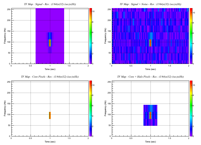
- resolution with 16 layers

- resolution with 32 layers

The whitening
The procedure:
The TF samples are normalized by the noise RMS.
The RMS is calculated at the finest frequency resolution.
For each layer several values of the RMS are calculated by using the running average.

The window and stride parameters can be configured using the whiteWindow and the whiteStride parameters defined in user_parameters.C file, see ’2G conditioning’ in description of the parameters section.
Test2G_Whitening.C
is a full example which illustrates how the whitening works
Create simulated colored gaussian noise at 16384 Hz
Data are resampled to 4096 Hz
Initialize WDM used for whitening
Apply time frequency data transform at level=10 : pixel’s resolution is dt=250 ms - df=2 Hz
Plot strain data samples distribution -> Strain data samples distribution
Plot strain PSD data -> Strain data PSD
Initialize WDM used for whitening wseries::white
Whitening data
Plot nRMS data -> nRMS TF data
Plot whitened data TF amplituded -> “Whiten data TF sqrt((E00+E90)/2)
Plot whitened data distribution & Fit with a gaussian -> Whitened WDM coefficients distribution
Plot white PSD data -> Whitened data PSD
Plot Average and RMS of the whitened data -> AVR (black )RMS (red) of the whitened data
If #define USE_GAUS_NOISE is declared the macro produces the plots for gaussian noise:


The pixels selection
The procedure:
For each WDM resolution the excess power (hot, black) pixels are selected for the subsequent analysis. First, the energy TF maps are created for each detector by using the wseries::maxEnergy function. Then the network pixel energy network::THRESHOLD is calculated. And finally the black pixels are selected in network::getNetworkPixels The main difference between the 1G and 2G algorithms for selection of black pixel is that in cWB2G the non-local selection rule is used : a pixel is selected if its energy is greater than some threshold (local rule) and the energy of neighbor pixels is above some (second) threshold (non-local rule).
In the following description we show step by step how the pixels selection works, using as an example an NSNS signal at the time-frequency resolution dt=250ms, df=2Hz with gaussian noise.
Whitening : The data are whitened.
- whitened L1 data

- whitened H1 data

- whitened V1 data

Max Energy : The function wseries::maxEnergy creates a time frequency map of maximum of energy over sky dependent time shifts. That is for each time-frequency wavelet pixel, try out many shift within +/-dT and save the largest obtained energy. The shifting is done using the cpf function that shift only by positive number of samples, and has a different syntax for forward and backward shifting. The zero and last layer are zeroed out. ( Note : The 0 parameter in Forward means the computed TF map contains energy not amplitude)
- max energy L1 data

- max energy H1 data

- max energy V1 data

Threshold : The function network::THRESHOLD computes a threshold on the energy of pixels that are called black (used for clustering), which should correspond to a fraction of all the TF pixels. A heuristic is used that combines the expectation from Gaussian noise, and the actual energy in the TF map (the energy is summed over the detectors in the network). The input from the energy TF map are robust estimate such as the median, the actual threshold for getting 10 times and 1 times the required fraction of pixels. The logic is that we don’t want some loud glitch to blind the analysis of the whole segment, but also to limit the total number of processed pixels when the noise is non-Gaussian.
print out in the coherence stage
-------------------------------------------------------------------------------------------
setup
-------------------------------------------------------------------------------------------

segment length                  = 192 sec
same rate                       = 1024 Hz
decomposition levels            = 3,4,5,6,7,8
number of pixels                = 192*1024 = 196608
bpp                             = 0.001
number of pixels to be selected = 196608*0.001 ~ 196

-------------------------------------------------------------------------------------------
legend
-------------------------------------------------------------------------------------------

m           : corrective factor for Gamma function : Gamma(N*m,x)
M       : number of frequency levels
bpp         : black pixels probability
0.2(D)      : threshold of the 20% of loudest data pixels
0.2(G)      : threshold of the 20% probability (Gamma function)
0.01(D)     : threshold of the  1% of loudest data pixels
0.01(G)     : threshold of the  1% probability (Gamma function)
bpp(D)      : threshold of the bpp of loudest data pixels
bpp(G)      : threshold of the bpp probability (Gamma function)
N*log(m)    : corrective threshold value (N=number of detectors)
fff     : (number of data pixels with energy > 0.0001)/(total pixels)

-------------------------------------------------------------------------------------------
level : 8        rate(hz) : 4    layers : 256    df(hz) : 2      dt(ms) : 250
-------------------------------------------------------------------------------------------

m       M       bpp     0.2(D)  0.2(G)  0.01(D) 0.01(G) bpp(D)  bpp(G)  N*log(m)  fff
1.08    257     0.001   4.572   4.579   8.990   8.809   13.034  11.681  0.231     0.965

thresholds in units of noise variance: Eo=7.64537083516 Em=15.29074167032

SELECTED PIXELS : 254

-------------------------------------------------------------------------------------------
level : 7        rate(hz) : 8    layers : 128    df(hz) : 4      dt(ms) : 125
-------------------------------------------------------------------------------------------

m       M       bpp     0.2(D)  0.2(G)  0.01(D) 0.01(G) bpp(D)  bpp(G)  N*log(m)  fff
1.17    129     0.001   4.890   4.914   9.371   9.254   13.445  12.179  0.471     0.961

thresholds in units of noise variance: Eo=8.1584324453822 Em=16.316864890764

SELECTED PIXELS : 221

-------------------------------------------------------------------------------------------
level : 6        rate(hz) : 16   layers : 64     df(hz) : 8      dt(ms) : 62.5
-------------------------------------------------------------------------------------------

m       M       bpp     0.2(D)  0.2(G)  0.01(D) 0.01(G) bpp(D)  bpp(G)  N*log(m)  fff
1.32    65      0.001   5.448   5.466   9.973   9.981   14.149  12.991  0.833     0.954

thresholds in units of noise variance: Eo=8.9750179277537 Em=17.950035855507

SELECTED PIXELS : 221

-------------------------------------------------------------------------------------------
level : 5        rate(hz) : 32   layers : 32     df(hz) : 16     dt(ms) : 31.25
-------------------------------------------------------------------------------------------

m       M       bpp     0.2(D)  0.2(G)  0.01(D) 0.01(G) bpp(D)  bpp(G)  N*log(m)  fff
1.57    33      0.001   6.350   6.374   11.070  11.159  15.249  14.300  1.353     0.939

thresholds in units of noise variance: Eo=10.21794047063 Em=20.435880941261

SELECTED PIXELS : 190

-------------------------------------------------------------------------------------------
level : 4        rate(hz) : 64   layers : 16     df(hz) : 32     dt(ms) : 15.625
-------------------------------------------------------------------------------------------

m       M       bpp     0.2(D)  0.2(G)  0.01(D) 0.01(G) bpp(D)  bpp(G)  N*log(m)  fff
1.93    17      0.001   7.653   7.659   12.435  12.797  16.503  16.111  1.973     0.882

thresholds in units of noise variance: Eo=11.756692941231 Em=23.513385882461

SELECTED PIXELS : 171

-------------------------------------------------------------------------------------------
level : 3        rate(hz) : 128  layers : 8      df(hz) : 64     dt(ms) : 7.8125
-------------------------------------------------------------------------------------------

m       M       bpp     0.2(D)  0.2(G)  0.01(D) 0.01(G) bpp(D)  bpp(G)  N*log(m)  fff
2.4     9       0.001   9.294   9.308   14.203  14.859  17.851  18.378  2.626     0.778

thresholds in units of noise variance: Eo=13.494924381499 Em=26.989848762999

SELECTED PIXELS : 119
Pixel Selection : The function network::getNetworkPixels selects the pixels from the sum over detectors energy TF map. There are two threshold: E0 and Em=2*Eo. To be selected a pixel needs to be either above Em by itself, or be above E0 and above Em when making a geometric mean with some neighboring pixels. The neighboring pixels considered in a 5x5 matrix around the pixel, and are grouped into 4 wedges of 3 pixels in the upgoing-chirp direction. The geometric mean is done between the considered pixel and the sum of energy in two consecutive wedges. Very loud pixels are trimmed to Em+0.1 to not over-select their neighbors, the energy of vetoed pixels is reset to 0.
- the non local rule selection scheme

- network max energy data

- selected network max energy data
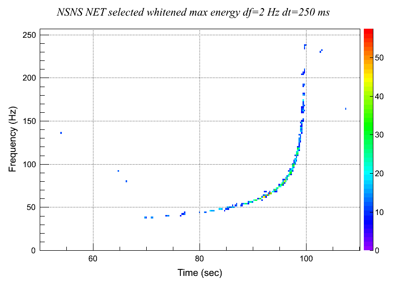
The sub-net cut algorithm
The cWB2G pipeline has two stages: ETG (generation of triggers) and Likelihood (reconstruction of GW events). The ETG stage is organized in the following way:
read data, data quality
produce TF maps withWDM transform, data conditioning
selection of excess power pixels for multiple TF resolutions, store pixel files for each time lag.
cluster and super-cluster analysis - the cWB2G triggers are formed
calculation of time delay arrays and sub-network cut, which main purpose is to reduce the ETG output pixel rate
selected triggers and the corresponding sparse TF maps are stored in the trigger files.
The main idea of the sub-network cut is to get rid of the single detector glitches which dominate the ETG rate. The algorithm is based on the sub-network energy e-e[k], where e is the total network energy and e[k] is the energy in the detector k. The subNetCut function performs the following steps :
calculate the amplitude time delay arrays for each pixel and each detector. The delayed amplitudes are calculated in the interval [-Tnet, Tnet] with the time step of 1/sampling rate (Tnet is maximum propagation time between detectors). The amplitude array represents amplitudes in a given pixel (and detector) if data is shifted by some time delay tau. So each network pixel contains K delayed amplitude arrays, one per detector, where K is the number of detectors in the network.
The delay amplitudes are calculated only for first LOUD pixels in the event (LOUD is a production parameter and a typical value is 300). If a trigger has <300 pixels it is not affected by this parameter. If number of pixels in the trigger >LOUD, only first LOUD pixels has the amplitude array initialized.
Perform loop over the sky with sparse segmentation (HEALPIX=4). In each sky point first, network pixels are selected if their total energy e>En. The threshold En = 2*K*Ao*Ao, where Ao=1.5-1.7 (is amplitude in units of the detector noise rms : Ao=Acore where Acore is a production parameter).
Then the total energy Eo=sum{e} and the minimum sub-network energy Ls=sum{min{e-e[k]}} are calculated. The sums are performed over all selected network pixels : the number of these pixels is N.
In addition, the reduced sub-network energy Ln is calculated in the same way as Ls, but dropping the terms min{e-e[k]} if they are below the threshold Es. The number of pixels M in the Ln sum is M<N. The threshold Es is uniquely defined by the En : Es is the threshold for K-1 network as opposed to En which is for K detectors.
The statistic aa = Ls*Ln/(Eo-Ls) is calculated. For injections aa is ~Ls and the factor Ln/(Eo-Ls) penalizes glitches. If (aa-M)/(aa+M)<subcut (subcut is a production parameter, default is 0.33) the sky location is not considered for the further analysis. Number of pixels M serves as a rough estimate of the null energy. Therefore this condition in the skyloop compares the subnetwork energy with the “null” energy of the event.
For the selected sky locations (the ones which pass the previous step) a more accurate estimate of the null energy is performed: “NULL” = (Eo-Lo)+2*N*(Eo-Ln)/Eo where Eo is total energy and Lo is reconstructed energy. The sky location with max aa/(aa+”NULL”) is selected.
The event is accepted if aa/(aa+”NULL”) is above some threshold (subnet) and the reconstructed energy per detector Lo/K is above netRHO^2: the subnet and netRHO are the production cWB2G parameters
The subnetwork cut allows us to reduce the output ETG rate by a factor of 50-100
More aggressive selection of triggers is possible, but it will require more detailed tuning of the subNetCut parameters
All subNetCut thresholds (En, Es, subnet, subcut, netRHO) are selected such that they do not affect the final cWB2G performance. The final detection efficiency is determined by the postproduction cuts. However, a small fraction of events, even with large SNR is lost when most of the network energy is concentrated in one detector. This is inevitable loss, because we can not claim a detection for such events. Typical loss of high SNR events due to subNetCut is few % and usually much less than the loss due to the regulators.
There are several limitations:
LOUD parameter: if increased it may crash cWB2G jobs due to excessive memory allocation
time delay segmentation of the amplitude arrays and sky segmentation. For nominal delay and sky segmentation the ETG stage is not computationally feasible.
Also delay and sky segmentation do not allow us to use coherent statistics (coherent energy) which limits the reduction factor for the pixel rate.
The cWB 2G clustering algorithms
Once a list of excess power pixels (pixel structure is described by the netpixel class is selected, the next step is to identify burst events. In cWB, the events are defined as groups of pixels (clusters) in the time-frequency data. The pixel list is stored in the cwb_library:netcluster class, which contains cluster metadata and methods to handle clusters. The only clustering condition is proximity of TF pixels in time and frequency. There are three different types of clusters:
- single TF resolution clusters
a simple clustering algorithm is used to structure a list of pixels into a linked list, with initialized pointers to the neighbor pixels. The single TF resolution pixels are neighbors, if they are adjacent in frequency or time. The neighbors are set by cwb_library:netcluster::cluster function, where n and m are gaps in units of pixels for time and frequency. In the cWB2G n=m=1 - two nearby pixels are clustered if the gaps do not exceed one pixel. The clustering metadata is set in cwb_library:netcluster::cluster() function and the clustering algorithm is implemented in the recursive cwb_library:netcluster::cluster(netpixel) function - these functions have not been changed since the S5/S6 analysis.
- superclusters
(netcluster::supercluster) combine single TF clusters from different resolutions in a supercluster. The clustering condition is defined by a single dimensionless “proximity” threshold gap (default value of 6). To maintain the backward compatibility with the S5/S6 analysis the 2G supercluster is implemented as a separate function. In 2G analysis the supercluster algorithm is complemented with the defragmentation function, which combines nearby superclusters into a single event. The defragmentation condition is defined by 2 thresholds: Tgap [sec] and Fgap [Hz] (see cluster thresholds).
- monster cluster analysis
(monster class and network::_sse_MRA_ps function in the network class) extract principal components (subset of TF pixels from different resolutions) from the oversampled pixel set. The extracted pixel amplitudes are used for the event reconstruction (waveforms and sky location). To perform the MCA, the overlap integrals of basis functions from different TF resolutions should be calculated - a set of overlap integrals define the overlap catalog.
How to create a catalog using the monster class :
CreateOverlapCatalog.C
- Test of the monster classAs an example we used white noise sampled at 1024Hz and produced two time-frequency maps: ( )

Next, using the overlap coefficients computed by the monster class we subtract each pixel in the first TF map from the second. Since the two TF maps represent the same signal, ideally the subtraction would remove all the energy. However, this is never the case since we only store overlap coefficients = 0.01: ( )

The plot above, after the subtraction, shows that over 99.9% of the energy has been removed, as expected. We conclude that the overlap (“cross-talk”) coefficients are computed correctly by the monster class. ( )
 The script for this test is available in the repository:
reviewMonster.C
The standard FAD statistic
NOTE : this documentation is extract from Giulio Mazzolo PhD thesis 2013
It is convenient to perform searches on multiple networks and combine the results of the analyses into one single measurement. In general, however, different searches do not share similar sensitivities. The differences in sensitivity could arise from the considered networks, epochs and data-analysis methods. The FAR statistic does not enable a direct comparison and combination of searches showing different sensitivities. The FAR encodes only information on the background affecting the analysis. The FAD statistic is defined as : In the above equation, \( T_{bkg} \) is the effective background livetime, \( V_{vis} \) is the \( V_{vis} \) averaged over the tested parameter space and the sum runs over the background events louder than a specific value. The FAD measures the density of false alarms within the \( V_{vis} \) in which the analysis is sensitive to the investigated GW source. With the introduction of the FAD, the information of how noisy the search is, the background, includes now the search sensitivity as well. As a rough approximation, in fact, the FAD statistic can be thought of as a weighted FAR, the weight being the visible volume surveyed by the search. GW candidates reconstructed by different searches are compared and ranked in terms of the FAD statistic. Louder events are characterized by lower FAD values. In particular, it is possible to compare in terms of FAD events reconstructed by different data-analysis algorithms. This is a desirable property since, in general, different algorithms do not share common ranking statistics. To compute the significance of a GW candidate, the FAD of the event is compared to the search productivity The productivity measures the space-time 4-volume surveyed by the combined searches and is defined as : In the above equation, the sum runs over K combined searches and \(V_{\text{vis}, \, k} \, (\text{FAD})\) is the visible volume surveyed at the desired FAD. \(V_{\text{vis}, \, k} \, (\text{FAD})\) is evaluated by applying the \(\eta^*\) cut on the simulation study such that \(\text{FAD}(\eta^*)\) is the desired FAD. The expected mean number of events originated by the noise sources within the 4-volume (FAD) is calculated as : Finally, assuming the background to be Poisson-distributed, the probability that a background process could originate N events at FAD lower than FAD is calculated as : It is straightforward to note that the approach developed in this section is the extension of the formalism used for the FAR :
Further documents :
S. Klimenko and C.Pankow, Detection statistic for multiple algorithms, networks and data sets, LIGO note T-1300869, pdf
Search for gravitational waves from intermediate mass black hole binaries, C.Pankow Thesis 2011
The Qveto
The all-sky burst search is covering a vast parameter space of anticipated GW signals. We do not know how they populate the parameter space, but we know how detector glitches do that. Similar to the CBC high mass and IMBBH searches which divide the parameter space of binary events into mass and spin bins, the all-sky search can divide the parameter space in duration, bandwidth and q-factor bins. The point of this division is to rank events in each bin independently. Therefore, FAR of GW candidates in each bin is calculated with respect to the corresponding background. Bins affected by background will yield low detection significance, while significance of events in the quiet bins will be enhanced. The purpose of Qveto is to separate all-sky search triggers into a “clean“ and “dirty“ samples based on the quality factor of the events. This selection rule does not really reject events as background, but rather tags them into different classes. Qveto is not the only selection rule like that - in general, additional selection rules are anticipated: a) selection rule based on the duration of events to identify a sample of “long duration” bursts (so called long duration search) and b) the selection rule based on the bandwidth to mitigate glitches coming from non-stationary lines.
cWB_Plugin_Qveto.C
In the following we describe the procedure to compute the Qveto.

The computation of the Qveto is defined by two parameters :
The parameter NTHR is used to select the number of relative maximum around the maximum value.
The parameter ATHR is used to exclude signal noise
The list of steps used in the procedure are the following :
the amax amplitude
1 amplitude on the left of the amax value
1 amplitude on the right of the amax value
select the green amplitudes (Ag) according the ATHR
Ag are the amplitudes with |Ag|>|amax|/ATHR
compute the Qveto :
Qveto = Eg / Eb = Sum[Ag*Ag] / Sum[Ab*Ab]
The Qveto is computed for nIFO reconstructed waveforms and nIFO whitened waveforms (signal+noise), the minimum of the 2*nIFO Qveto values is stored in the output root file in the first element of the array Qveto[2].Beside the Qveto it is also estimated the Qfactor.
R = ( max_left_peak+max_right_peak ) / 2 / max_main_peak max_main_peak = absolute value of the max main peak max_left_peak = absolute value of the max left peak nearest to the main peak max_right_peak = absolute value of the max right peak nearest to the main peak
Qfactor is stored in Qveto[1]
The default values used in
cWB_Plugin_Qveto.C
are :
NTHR = 1
ATHR ~ 7.6
Such values have been empirically selected based on tests done with the advanced detectors background.
The separation of the all-sky search triggers into a “clean“ and “dirty“ sets is done in the post-production phase according to the following rule :
clean set : (Qveto[0]>QTHR0 && Qveto[1]>QTHR1)
dirty set : !(Qveto[0]>QTHR0 && Qveto[1]>QTHR1)
where :
QTHR1 and QTHR2 are used to select the max Q factor of the glitches
The Lveto
There are very narrow-band glitches (few Hz) mainly observed at the power line frequencies and near dither lines. The Lveto algorithm is used to identify such glitches and compute additional parameters to be added to the event data record. The LVeto code is implemented as a plugin :
cWB_Plugin_Qveto.C
The output of the plugin is used for an additional selection cut designed to reduce FAR from the narrow-band glitches.
In the following we describe the procedure to compute the Lveto. The
figure shows the time-frequency principal component pixels of the
reconstructed signal. These pixels are used by the plugin to identify
the Lveto glitch parameters.
|
|  |
|
The list of steps used in the procedure are the following :
- the code looks for the pixel with the maximum energy and save the
following parameters :
1) the central frequency of the max pixel : freq_max_pixel
2) the frequency width of the max pixel : width_max_pixel
all pixels with central frequency in the frequency range :
pix_freq_range = [freq_max_pixel-width_max_pixel : freq_max_pixel+width_max_pixel]are used to compute the following parameters :
the frequency mean
the frequency rms
the energy in the pix_freq_range
The parameters are stored into the event data record into the array Lveto[3] :
Lveto[0] = the frequency mean
Lveto[1] = the frequency rms
Lveto[2] = the energy ratio of the energy in the pix_freq_range and the total energy of the event
If Lveto[2] is near to 1 then most of the signal energy is inside the Lveto[0]+/-Lveto[1] range and Lveto[1] can be used to identify the narrow-band glitches.
The Gating Plugin
Gating is the procedure to mitigate the data quality issues associated with very loud glitches in data. The super-glitches affect calculation of the cWB threshold making it very large. As a result, the job segments with super-glitches are insensitive to GW and produce high-SNR glitches. | The plugin which implements the gating is
cWB_Plugin_Gating.C
It is executed in the 2G pipeline class cwb2G at the beginning of the COHERENCE stage before the time-frequency maps of the max energies used for (the pixels selection).

Gating excludes from the analysis all pixels in a time interval where there is a super-glitch.
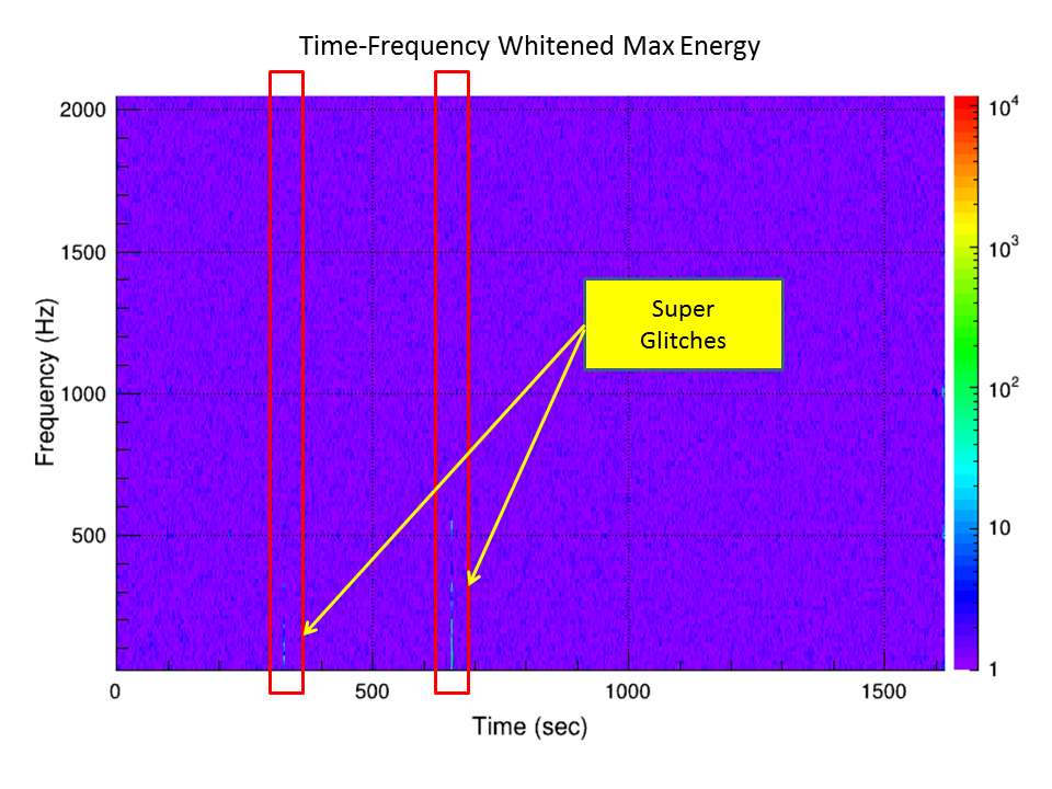
The Procedure
The procedure is applied for each detector.
The list of steps used in the
cWB_Plugin_Gating.C
are the following :
- The time-frequency map of the whitened max energies is projected on the time axis.
For each time index is computed the sum of the pixel energy over all frequency layers.
- Apply a moving average window.
The time whitened energy samples are integrated over the time window
- TWIN.
The parameter TWIN must be selected as the maximum time length of the super-glitches that must be excluded from the analysis.
- Find the time samples to be excluded from the selection
A time sample is marked as to be excluded when the time integrated energy is greater than SETHR When a time sample is excluded also the time samples in the interval
- [sample-TEDG:sample+TEDG] are also excluded.
These pixels do not participate in the computation of the pixel’s selection threshold and are excluded from the selection
- Merge segments lists
The vetoed segments of all detectors are merged in a unique segments list

The default values used in
cWB_Plugin_Gating.C
are :
- SETHR = 1000000
The events which are excluded by this threshold are the ones with
SNRdet>sqrt(SETHR)=1000 in at least one detector.
TWIN = 0.5 sec
TEDG = 1.5 sec
The WDM packets
pdf - What_are_wavelet_packets.pdf
The signal reconstruction and regulators (WP)
pdf - Signal_reconstruction_and_regulators.pdf